TMM4175 Polymer Composites

Home About Python Links Table of Contents

Micro-mechanical models¶

Micro-mechanical models atempt to estimate the properties of composites based on the geometrical arrangement and the properties of the constituent materials in the composite material. The most simple models are typically based on a rule of mixture where assumtions of parallel or series coupling are being made.

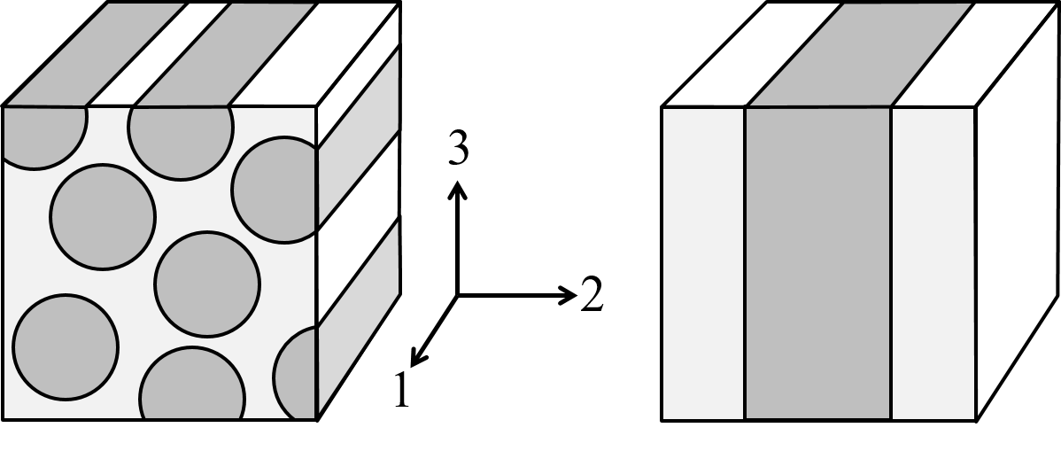
Figure-1: Simplified model of a UD composite

Longitudinal modulus¶

We can reasonably assume that the longitudinal strain in the fiber is equal to the longitudinal strain in the matrix, and both strains are equal to the longitudinal strain of the composite:

$\begin{equation} \varepsilon_{1f} = \varepsilon_{1m} = \varepsilon_1 \tag{1} \end{equation}$

When subjected to a longitudinal force $F_1$ , this force is distributed between the fiber and the matrix:

$\begin{equation} F_1 = F_{1f}+F_{1m} \tag{2} \end{equation}$

Taking the cross section areas into consideration, the longitudinal stresses are introduced:

$\begin{equation} A \sigma_1 = A_f \sigma_{1f} + A_m \sigma_{1m} \tag{3} \end{equation}$

or

$\begin{equation} \sigma_1 = \frac{A_f}{A} \sigma_{1f} + \frac{A_m}{A} \sigma_{1m} = V_f \sigma_{1f} + V_m \sigma_{1m} \tag{4} \end{equation}$

where the relations between volume fractions and area fractions have been used.

Now dividing by the strain: $\begin{equation} \frac{\sigma_1}{\varepsilon_{1}} = V_f \frac{\sigma_{1f}}{\varepsilon_{1}} + V_m \frac{\sigma_{1m}}{\varepsilon_{1}}=V_f \frac{\sigma_{1f}}{\varepsilon_{1f}} + V_m \frac{\sigma_{1m}}{\varepsilon_{1m}} \tag{5} \end{equation}$

and by applying the definition of modulus:

$\begin{equation} E_1 = V_f E_{f1} + V_m E_m \tag{6} \end{equation}$

or

$\begin{equation} E_1 = V_f E_{f1} + (1-V_f) E_m \tag{7} \end{equation}$

This model is considered to be very accurate for most of the common combinations of fibers and polymer matrices.

Example:

Ef=70            # Modulus for E-glass fiber
vf=0.2           # Poisson's ratio for glass
Gf=Ef/(2+2*vf)   # Derived shear modulus assuming isotropy
Em=3             # Modulus for a polymer matrix
vm=0.4           # Poisson's ratio for the matrix
Gm=Em/(2+2*vm)   # Derived shear modulus assuming isotropy

Vf=0.5           # Fiber volume fraction

E1=Vf*Ef + (1-Vf)*Em

print('E1=',E1)

E1= 36.5

The expression (7) is frequently called the upper-bound value for the modulus when mixing two materials. This term is however not completly consistent since the real upper-bound value is found by using the rule of mixture to the stiffness matrices of the to constituents as demonstrated below. The real upper-bound modulus is eventually found from the mixed compliance matrix. Note that the difference is minor for this case (36.9 versus 36.5) and typically within the error of experiments.

import numpy as np

Sf = np.array([[1/Ef,-vf/Ef,-vf/Ef,0,0,0],       # Compliance matrix of the (isotropic) fiber
               [-vf/Ef,1/Ef,-vf/Ef,0,0,0],
               [-vf/Ef,-vf/Ef,1/Ef,0,0,0],
               [0,0,0,1/Gf,0,0],
               [0,0,0,0,1/Gf,0],
               [0,0,0,0,0,1/Gf] ])

Sm = np.array([[1/Em,-vm/Em,-vm/Em,0,0,0],       # Compliance matrix of the (isotropic) matrix
               [-vm/Em,1/Em,-vm/Em,0,0,0],
               [-vm/Em,-vm/Em,1/Em,0,0,0],
               [0,0,0,1/Gm,0,0],
               [0,0,0,0,1/Gm,0],
               [0,0,0,0,0,1/Gm] ])

Cf = np.linalg.inv(Sf)   # Stiffness matrix of fiber
Cm = np.linalg.inv(Sm)   # Stiffness matrix of matrix

C = Vf*Cf + (1-Vf)*Cm    # Rule of mixture stiffness matrix

S = np.linalg.inv(C)     # Compliance matrix from rule of mixture stiffness matrix

E1 = 1/S[0,0]

print('E1=',E1)

E1= 36.88602941176471

Transverse modulus¶

In the simplest model for the transverse modulus, we assume a series coupling of fibers and matrix where the resulting strain in the transverse direction is a superposition of the fiber strain and the matrix strain, while the stress in the two phases are equal. The resulting model gives

$\begin{equation} \frac{1}{E_2} = \frac{V_f}{E_{f2}} + \frac{1-V_f}{E_m} \tag{8} \end{equation}$

or

$\begin{equation} E_2 = \frac{E_{2f} E_m}{V_f E_m + V_m E_{2f} } \tag{9} \end{equation}$

NOTE: Glass fibers are isotropic while carbon, kevlar and other polymer fibers are anisotropic. The transverse modulus of for example carbon fibers is just a fraction of the longitudinal modulus, from 1/20 to 1/50, dependent on the type of carbon fiber.

Example:

E2=1/(Vf/Ef + (1-Vf)/Em)

print('E2=',E2)

E2= 5.7534246575342465

The model (9) provides a fair estimate of the property but tends to underestimate the value significantly since it is the true lower-bound value where constraints due to Poisson's effects are completly neglected. One simple approach for mitigating this issue suggests the modulus of the matrix be modified to

$\begin{equation} E_m'=\frac{E_m}{1-\nu_m^2} \tag{10} \end{equation}$

where $\nu_m$ is the Poisson's ratio of the matrix.

Hence, the modified model can be expressed by

$\begin{equation} E_2 = \frac{E_{2f} E_m'}{V_f E_m' + V_m E_{2f} } \tag{11} \end{equation}$

Example:

Emm=Em/(1-vm**2)
E2=(Ef*Emm)/(Vf*Emm + (1-Vf)*Ef)

print('E2=',E2)

E2= 6.7961165048543695

Note that expression (8) is simply the rule of mixture to the compliance matrices of the to constituents as demonstrated below.

S = Vf*Sf + (1-Vf)*Sm    # Rule of mixture of compliance matrices

E1 = 1/S[0,0]

print('E1=',E1)

E1= 5.7534246575342465

The semi-empircal Halpin-Tsai model for the transverse modulus is

$\begin{equation} E_2 = E_m\frac{1+\xi_1 \eta_1 V_f}{1-\eta_1 V_f} \tag{12} \end{equation}$

where $\begin{equation} \eta_1 = \frac{E_{2f}-E_m}{E_{2f}+\xi_1 E_m} \tag{13} \end{equation}$

and $\xi_1$ is an experimentally determined parameter which typically lay between 1 and 2.

Since the emperical parameter must be determined, the model is only useful for predicting the elastic constants for a given fiber volume fraction when it is known for another fiber volume fraction.

Examples: The model predictions as function of the fiber volume fraction for a UD glass fiber composite:

def micmec_E1(Vf,E1f,Em):
    return Vf*E1f+(1-Vf)*Em

def micmec_E2a(Vf,E2f,Em):
    return (E2f*Em)/(Vf*Em + (1-Vf)*E2f)

def micmec_E2b(Vf,E2f,Em,vm):
    Emm=Em/(1-vm**2)
    return (E2f*Emm)/(Vf*Emm + (1-Vf)*E2f)

def micmec_E2c(Vf,E2f,Em,xi1):
    n1=(E2f-Em)/(E2f+xi1*Em)
    return Em*(1+xi1*n1*Vf)/(1-n1*Vf)

import numpy as np

Vf=np.linspace(0,1.0)

E1 =  micmec_E1(Vf,70,3)
E2a = micmec_E2a(Vf,70,3)
E2b = micmec_E2b(Vf,70,3,0.4)
E2c1 = micmec_E2c(Vf,70,3,1.0)
E2c2 = micmec_E2c(Vf,70,3,2.0)

import matplotlib.pyplot as plt
%matplotlib inline

fig,(ax1,ax2) = plt.subplots(nrows=1,ncols=2,figsize=(12,4))

ax1.plot(Vf,E1, color='black',label=r'$E_1$')
ax1.plot(Vf,E2a, color='blue',label=r'$E_2^{(a)}$')
ax1.plot(Vf,E2b, color='red',label=r'$E_2^{(b)}$')
ax1.plot(Vf,E2c1, color='orange',label=r'$E_2^{(c)}, \xi_1 = 1$')
ax1.plot(Vf,E2c2, color='cyan',label=r'$E_2^{(c)}, \xi_1 = 2$')
ax1.set_xlim(0,1)
ax1.set_ylim(0,)
ax1.set_xlabel('Fiber Volume Fraction',size=12)
ax1.set_ylabel('Modulus [MPa]',size=12)
ax1.grid(True)
ax1.legend(loc='best')

ax2.plot(Vf,E2a, color='blue',label=r'$E_2^{(a)}$')
ax2.plot(Vf,E2b, color='red',label=r'$E_2^{(b)}$')
ax2.plot(Vf,E2c1, color='orange',label=r'$E_2^{(c)},\xi_1 = 1$')
ax2.plot(Vf,E2c2, color='cyan',label=r'$E_2^{(c)},\xi_1 = 2$')
ax2.set_xlim(0.4,0.7)
ax2.set_ylim(0,15)
ax2.set_xlabel('Fiber Volume Fraction',size=12)
ax2.set_ylabel('Modulus [MPa]',size=12)
ax2.grid(True)
ax2.legend(loc='best')
plt.tight_layout()

Poisson's ratio¶

A model for the Poisson's ratio $v_{12}$ similar to the model for longitudinal modluls $E_1$ has been found to be very close to experimental results:

$\begin{equation} v_{12} = V_f v_{12f} + (1-V_f) v_m \tag{14} \end{equation}$

Models for the Poisson's ratio $v_{23}$ tend to be rather involved, and will not be considered further in this course.

Shear modulus¶

The simple rule of mixture similar to equation (9) for the transverse modulus provides an estimate for the composite shear modulues:

$\begin{equation} G_{12} = \frac{G_{12f} G_m}{V_f G_m + V_m G_{12f} } \tag{15} \end{equation}$

The Halpin-Tsai semi-empirical model is

$\begin{equation} G_{12} = G_m\frac{1+\xi_2 \eta_2 V_f}{1-\eta_2 V_f} \tag{16} \end{equation}$

where $\begin{equation} \eta_2 = \frac{G_{12f}-G_m}{G_{12f}+\xi_2 G_m} \tag{17} \end{equation}$

and $\xi_2$ is an experimentally determined parameter.

Functions:

def micmec_v12(Vf,v12f,vm):
    return Vf*v12f+(1-Vf)*vm

def micmec_G12a(Vf,G12f,Gm):
    return (G12f*Gm)/(Vf*Gm + (1-Vf)*G12f)

def micmec_G12c(Vf,G12f,Gm,xi2):
    n2=(G12f-Gm)/(G12f+xi2*Gm)
    return Gm*(1+xi2*n2*Vf)/(1-n2*Vf)

Gm=3/(2+2*0.4)
G12f=70/(2+2*0.22)

G12a = micmec_G12a(Vf,G12f,Gm)
G12c = micmec_G12c(Vf,G12f,Gm,1)

fig,(ax1,ax2) = plt.subplots(nrows=1,ncols=2,figsize=(12,4))

ax1.plot(Vf,G12a, color='blue',label=r'$G_{12}^{(a)}$')
ax1.plot(Vf,G12c, color='orange',label=r'$E_{12}^{(c)}, \xi_1 = 1$')
ax1.set_xlim(0,1)
ax1.set_ylim(0,)
ax1.set_xlabel('Fiber Volume Fraction',size=12)
ax1.set_ylabel('Modulus [MPa]',size=12)
ax1.grid(True)
ax1.legend(loc='best')

ax2.plot(Vf,G12a, color='blue',label=r'$G_{12}^{(a)}$')
ax2.plot(Vf,G12c, color='orange',label=r'$G_{12}^{(c)},\xi_1 = 1$')
ax2.set_xlim(0.4,0.7)
ax2.set_ylim(0,5)
ax2.set_xlabel('Fiber Volume Fraction',size=12)
ax2.set_ylabel('Modulus [MPa]',size=12)
ax2.grid(True)
ax2.legend(loc='best')
plt.tight_layout()

Thermal expansion¶

Left as exercise.

References and further readings¶

Herakovich, Carl T. Mechanics of Fibrous Composites. New York: Wiley, 1998.
Daniel, Isaac M., and Ori Ishai. Engineering Mechanics of Composite Materials. 2nd ed. New York: Oxford University Press, 2006.
Kollár, Lázló P., and George S. Springer. Mechanics of Composite Structures. Cambridge: Cambridge University Press, 2003.

Disclaimer:This site is about polymer composites, designed for educational purposes. Consumption and use of any sort & kind is solely at your own risk.
Fair use: I spent some time making all the pages, and even the figures and illustrations are my own creations. Obviously, you may steal whatever you find useful here, but please show decency and give some acknowledgment if or when copying. Thanks! Contact me: nils.p.vedvik@ntnu.no www.ntnu.edu/employees/nils.p.vedvik