TMM4175 Polymer Composites

Home About Python Links Table of Contents

Principles of failure prediction

Prediction of failure is accomplished using a failure criterion. A failure criterion is fundamentally a set of rules, functions or other expressions of logic that judges if a given state of loading will cause failure or not. For example, the Maximum stress criterion can be stated simply as: failure is predicted if any of the stress components exceeds the corresponding strengths.

A failure criterion is commonly expressed by a function that returns a numerical value that indicate failure or not. If the material is exposed to a state of stress $\boldsymbol{\sigma}$ and a set of strength parameters and optionally failure criterion parameters is $\Psi$, this is written generically as:

$$\begin{equation} f(\boldsymbol{\sigma},\Psi)=1 \Rightarrow \text{failure} \tag{1} \end{equation}$$

For any other outcomes we define:

$$\begin{equation} f(\boldsymbol{\sigma},\Psi) < 1 \Rightarrow \text{not failure} \tag{2} \end{equation}$$ $$\begin{equation} f(\boldsymbol{\sigma},\Psi) > 1 \Rightarrow \text{beyond failure} \tag{3} \end{equation}$$

Assume the most simple state of stress where $\sigma_1 > 0$ while all other stress components are zero. By the very definition of the failure strength $X_T$, failure shall be prediced when $\sigma_1 = X_T$. This is consistent with the function:

$$\begin{equation} f(\boldsymbol{\sigma},\Psi)=\frac{\sigma_1}{X_T} \tag{4} \end{equation}$$

Assume a slightly more complex state of stress where $\sigma_1>0$ and $\sigma_2 >0$ while the other stress components are zero. Now we must deal with the obvious question: How do the stresses interact? The Maximum stress criterion makes the simple assumption that there are no interactions, while several other criteria are base on quadratic interaction. A quadratic interaction can be expressed as:

$$\begin{equation} f(\boldsymbol{\sigma},\Psi) = \big( \frac{\sigma_1^2}{X_T^2} \big ) + \big( \frac{\sigma_2^2}{Y_T^2} \big ) = 1 \tag{5} \end{equation}$$

Solving for $\sigma_2$ as a function of $\sigma_1$ at failure yields:

$$\begin{equation} \big( \frac{\sigma_1^2}{X_T^2} \big ) + \big( \frac{\sigma_2^2}{Y_T^2} \big ) = 1 \Rightarrow \sigma_2 = Y_T \sqrt{ \Big( 1 - \big( \frac{\sigma_1^2}{X_T^2} \big ) \Big) } \tag{6} \end{equation}$$

The relation above can be visualized by creating a failure envelope of $\sigma_2$ versus $\sigma_1$ :

import matplotlib.pyplot as plt
import numpy as np
%matplotlib inline
fig,ax = plt.subplots(figsize=(6,3))
XT,YT=1000,100 # tensile strengths in 1 and 2 directions
s1 = np.linspace(0,XT,1000)
s2 = YT*( 1 - (s1/XT)**2 )**0.5
ax.plot(s1,s2,'--',color='blue',label='Max stress',linewidth=1)
ax.set_xlim(0,)
ax.set_ylim(0,)
ax.set_xlabel(r'$\sigma_1$',fontsize=14)
ax.set_ylabel(r'$\sigma_2$',fontsize=14)
ax.text(400,40,'No failure',fontsize=12)
ax.text(800,80,'Failure',fontsize=12)
ax.grid(True)
plt.tight_layout()
plt.show()

While the function

$$\begin{equation} f = \big( \frac{\sigma_1^2}{X_T^2} \big ) + \big( \frac{\sigma_2^2}{Y_T^2} \big ) \tag{7} \end{equation}$$

provides a predication of failure or not, the degree of exposure is somewhat hidden. Consider the following examples:

def f(s1,s2,XT,YT):
    return (s1/XT)**2 + (s2/YT)**2

print( f( s1=400, s2=30, XT=1000, YT=100 ) )
print( f( s1=800, s2=60, XT=1000, YT=100 ) )

0.25
1.0

The result for the two different state of stress are 0.25 and 1.0 respectively, where the stresses in the first case are exactly half of the stresses in the last case. Hence, the value 0.25 does not clearly suggest how much we could have increased the load before failure occures. Therefore, it is usefull to introduce the Load Proportionality Factor (LPF) . The LPF is the factor we can increase all loads (stress components) before failure. For the current example of a quadratic interaction between the two stress components:

$$\begin{equation} f(R\boldsymbol{\sigma},\Psi) = \big( \frac{R^2 \sigma_1^2}{X_T^2} \big ) + \big( \frac{R^2\sigma_2^2}{Y_T^2} \big ) = 1 \Rightarrow \frac{1}{R^2} = \big( \frac{\sigma_1^2}{X_T^2} \big ) + \big( \frac{\sigma_2^2}{Y_T^2} \big ) \tag{8} \end{equation}$$

where $R$ is the LPF.

The exposure factor (or frequently called the stress exposure factor) is

$$\begin{equation} f_E=\frac{1}{R} \tag{9} \end{equation}$$

such that

$$\begin{equation} f_E= \sqrt{ \big( \frac{\sigma_1^2}{X_T^2} \big ) + \big( \frac{\sigma_2^2}{Y_T^2} \big ) } \tag{10} \end{equation}$$

The exposure factor provides us with a convenient and straight forward quantity for failure assessment as explored in the following implementation:

def fE(s1,s2,XT,YT):
    return ( (s1/XT)**2 + (s2/YT)**2 )**0.5

print( fE( s1=400, s2=30, XT=1000, YT=100 ) )
print( fE( s1=800, s2=60, XT=1000, YT=100 ) )

0.5
1.0

The exposure factor $f_E$ can alternativly be found by iterations over the function $f(R\boldsymbol{\sigma},\Psi)$ as illustrated in the following example:

def fE_iteration(s1,s2,XT,YT):
    Rmax=1.0E6
    Rmin=0.0
    R=1.0
    err = 1.0
    conv = 0.0001
    while err > conv:
        f=(R*s1/XT)**2 + (R*s2/YT)**2
        if f > 1.0:
            Rmax=R
            R=(R+Rmin)/2.0
        if f < 1.0:
            Rmin=R
            R=(Rmax+R)/2.0
        err=abs(1.0 - f)
    print('fE=',1/R)

fE_iteration(400,30,1000,100)
fE_iteration(100,30,1000,100)

fE= 0.5000274516870216
fE= 0.316237571326712

In the first case ( $f_E = 0.5$) the material has been exposed to 50% of the capacity, meaning that all stresses could be increased twice before failure.

Summary

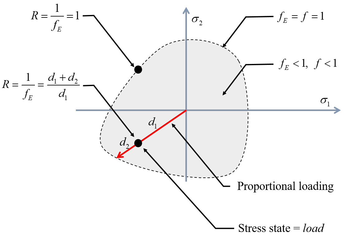
Figure-1: Interpretation of a failure envelope

Disclaimer:This site is about polymer composites, designed for educational purposes. Consumption and use of any sort & kind is solely at your own risk.
Fair use: I spent some time making all the pages, and even the figures and illustrations are my own creations. Obviously, you may steal whatever you find useful here, but please show decency and give some acknowledgment if or when copying. Thanks! Contact me: nils.p.vedvik@ntnu.no www.ntnu.edu/employees/nils.p.vedvik

Copyright 2021, All right reserved, I guess.