TMM4175 Polymer Composites

Home About Python Links Table of Contents

Effective properties of laminates

The effective properties, or homogenized properties, are useful for describing the behaviour of laminates in familiar enginering terms. That includes the effective elastic properties, bending and torsional stiffness, thermal expansion and laminate strength. The concept of effective properties are usually limited to symmetric and balanced laminates.

For symmetric laminates, $\mathbf{B}=\mathbf{0}$ and

$$\begin{equation} \begin{bmatrix} \mathbf{N} \\ \mathbf{M} \end{bmatrix}= \begin{bmatrix} \mathbf{A} & \mathbf{0} \\ \mathbf{0} & \mathbf{D} \end{bmatrix} \begin{bmatrix} \boldsymbol{\varepsilon^0} \\ \boldsymbol{\kappa} \end{bmatrix} \tag{1} \end{equation}$$

Hence, we can separate the in-plane relations from the out-of-plane relations;

$$\begin{equation} \mathbf{N} = \mathbf{A} \varepsilon^0 \tag{2} \end{equation}$$

and

$$\begin{equation} \mathbf{M} = \mathbf{D} \kappa \tag{3} \end{equation}$$

For a balanced laminate,

$$\begin{equation} \begin{bmatrix} N_x \\ N_y \\ N_{xy} \end{bmatrix} = \begin{bmatrix} A_{xx} & A_{xy} & 0 \\ A_{xy} & A_{yy} & 0 \\ 0 & 0 & A_{ss} \end{bmatrix} \begin{bmatrix} \varepsilon_x^0 \\ \varepsilon_y^0 \\ \gamma_{xy}^0 \end{bmatrix} \tag{4} \end{equation}$$

which can be separated into

$$\begin{equation} \begin{bmatrix} N_x \\ N_y \end{bmatrix} = \begin{bmatrix} A_{xx} & A_{xy} \\ A_{xy} & A_{yy} \\ \end{bmatrix} \begin{bmatrix} \varepsilon_x^0 \\ \varepsilon_y^0 \end{bmatrix} \tag{5} \end{equation}$$

and

$$\begin{equation} N_{xy} = A_{ss} \gamma_{xy}^0 \tag{6} \end{equation}$$

Effective in-plane elastic constants

Consider the load case $\quad N_x \ne 0 ,\quad N_y = 0$:

$$\begin{equation} N_x = A_{xx} \varepsilon_x^0 + A_{xy} \varepsilon_y^0 \tag{7} \end{equation}$$ $$\begin{equation} 0 = A_{xy} \varepsilon_x^0 + A_{yy} \varepsilon_y^0 \tag{8} \end{equation}$$

Combining (7) and (8) leads to

$$\begin{equation} N_x = \big ( A_{xx} - \frac{A_{xy}^2}{A_{yy}} \big) \varepsilon_x^0 \tag{9} \end{equation}$$

and

$$\begin{equation} -\frac{ \varepsilon_y^0}{\varepsilon_x^0 } =\frac{A_{xy}}{A_{yy}} \tag{10} \end{equation}$$

The resultant (average) stress $\bar \sigma_x$ is now

$$\begin{equation} \bar \sigma_x = \frac{N_x}{h}= \frac{1}{h} \big ( A_{xx} - \frac{A_{xy}^2}{A_{yy}} \big) \varepsilon_x^0 \tag{11} \end{equation}$$

where $h$ is the total thickness of the laminate.

The effective modulus $\bar E_x$ is therefore

$$\begin{equation} \bar E_x = \frac{1}{h} \big ( A_{xx} - \frac{A_{xy}^2}{A_{yy}} \big) \tag{12} \end{equation}$$

The left hand side of equation (10) is simply the definition of Poisson's ratio:

$$\begin{equation} v_{xy} =\frac{A_{xy}}{A_{yy}} \tag{13} \end{equation}$$

Correspondingly, when $\quad N_x = 0 ,\quad N_y \ne 0$, we can derive the modulus

$$\begin{equation} \bar E_y = \frac{1}{h} \big ( A_{yy} - \frac{A_{xy}^2}{A_{xx}} \big) \tag{14} \end{equation}$$

The effective in-plane shear modulus is obtained from equation (6):

$$\begin{equation} N_{xy} = A_{ss} \gamma_{xy}^0 \Rightarrow \bar G_{xy} = \frac{ \bar \tau_{xy}}{\gamma_{xy}^0} = \frac{1}{h} A_{ss} \tag{15} \end{equation}$$

Examples:

from laminatelib import laminateStiffnessMatrix, laminateThickness

# Material:
m1={'E1':140000, 'E2':10000, 'v12':0.3, 'G12':5000}

layup = [ {'mat':m1 , 'ori': 0   , 'thi':1} , 
          {'mat':m1 , 'ori': 90  , 'thi':1} ,
          {'mat':m1 , 'ori': 0   , 'thi':1}  ]

ABD = laminateStiffnessMatrix(layup)

h=laminateThickness(layup)

Ex = (1/h)*( ABD[0,0] - (ABD[0,1]**2)/ABD[1,1]  )
Ey = (1/h)*( ABD[1,1] - (ABD[0,1]**2)/ABD[0,0]  )
vxy = ABD[0,1]/ABD[1,1]
Gxy = (1/h)*ABD[2,2]

print('Ex=',Ex)
print('Ey=',Ey)
print('vxy=',vxy)
print('Gxy=',Gxy)

Ex= 97122.27414330219
Ey= 53584.702975615
vxy= 0.05624999999999999
Gxy= 5000.0

The effective elastic constants as function of $\theta$ for a laminate of type $[-\theta / +\theta / +\theta / -\theta]$:

theta,Ex,Ey,vxy,Gxy = [],[],[],[],[]

for i in range(0,90):
    layup = [ {'mat':m1 , 'ori': -i   , 'thi':1} , 
              {'mat':m1 , 'ori':  i   , 'thi':1} ,
              {'mat':m1 , 'ori':  i   , 'thi':1},
              {'mat':m1 , 'ori': -i   , 'thi':1}]
    ABD = laminateStiffnessMatrix(layup)
    h=laminateThickness(layup)    
    Ex.append(  (1/h)*( ABD[0,0] - (ABD[0,1]**2)/ABD[1,1]  )  )
    Ey.append(  (1/h)*( ABD[1,1] - (ABD[0,1]**2)/ABD[0,0]  )  )
    vxy.append( ABD[0,1]/ABD[1,1]  )
    Gxy.append( (1/h)*ABD[2,2]  )
    theta.append(i)

import matplotlib.pyplot as plt
%matplotlib inline

fig,(ax1,ax2) = plt.subplots(nrows=1,ncols=2, figsize = (12,4))
ax1.plot(theta,Ex,'--',color='red',label='$E_x$')
ax1.plot(theta,Ey,'-.',color='blue',label='$E_y$')
ax1.plot(theta,Gxy,'-',color='green',label='$G_{xy}$')
ax1.grid(True)
ax1.set_xlim(0,90)
ax1.legend(loc='best',prop={'size': 12})
ax1.set_xlabel(r'$\theta}$',size=12)
ax1.set_ylabel('Modulus',size=12)

ax2.plot(theta,vxy,'-',color='orange',label=r'$\nu_{xy}$')
ax2.grid(True)
ax2.set_xlim(0,90)
ax2.legend(loc='best',prop={'size': 12})
ax2.set_xlabel(r'$\theta}$',size=12)
ax2.set_ylabel('Poissons ratio',size=12)

plt.tight_layout()

plt.show()

Effective thermal properties

For a symmetric laminate:

$$\begin{equation} \begin{bmatrix} \mathbf{N} \\ \mathbf{M} \end{bmatrix}+ \begin{bmatrix} \mathbf{N}_{th} \\ \mathbf{M}_{th} \end{bmatrix}= \begin{bmatrix} \mathbf{A} & \mathbf{0} \\ \mathbf{0} & \mathbf{D} \end{bmatrix} \begin{bmatrix} \boldsymbol{\varepsilon}^0 \\ \boldsymbol{\kappa} \end{bmatrix} \tag{16} \end{equation}$$

When the external forces and moments are zero,

$$\begin{equation} \mathbf{N}_{th} = \mathbf{A}\boldsymbol{\varepsilon}^0 \tag{17} \end{equation}$$

Hence,

$$\begin{equation} \boldsymbol{\varepsilon}^0 = \mathbf{A}^{-1} \mathbf{N}_{th} \tag{18} \end{equation}$$

Then, by definition, the effective coefficients of thermal expansion for the laminate is

$$\begin{equation} \bar{\boldsymbol{\alpha}} = \boldsymbol{\varepsilon}^0 = \mathbf{A}^{-1} \mathbf{N}_{th},\quad\text{when} \quad \Delta T = 1 \tag{19} \end{equation}$$

Example:

from laminatelib import thermalLoad
import numpy as np

# Material:
m1={'E1':140000, 'E2':10000, 'v12':0.3, 'G12':5000, 'a1':-0.5E-6, 'a2':30.0E-6}

layup = [ {'mat':m1 , 'ori': 0   , 'thi':1} , 
          {'mat':m1 , 'ori':90   , 'thi':1} ,
          {'mat':m1 , 'ori': 0   , 'thi':1}  ]

ABD = laminateStiffnessMatrix(layup)

A=ABD[0:3,0:3]

Nth = thermalLoad(layup=layup,dT=1.0)[0:3]

effCTE =  np.dot(   np.linalg.inv(A),  Nth)

print(effCTE)

[ 1.04939658e-06  3.79722144e-06 -3.13924177e-21]

The following function computes the effective elastic properties as well as the effective coefficient of thermal expansion and return the results as a new material:

def laminateHomogenization(layup):
    ABD = laminateStiffnessMatrix(layup)
    h=laminateThickness(layup)
    Ex = (1/h)*( ABD[0,0] - (ABD[0,1]**2)/ABD[1,1]  )
    Ey = (1/h)*( ABD[1,1] - (ABD[0,1]**2)/ABD[0,0]  )
    vxy = ABD[0,1]/ABD[1,1]
    Gxy = (1/h)*ABD[2,2]
    (ax,ay,dummy) = np.dot( np.linalg.inv(ABD[0:3,0:3]), thermalLoad(layup,1.0)[0:3])
    return {'E1':Ex, 'E2':Ey, 'v12':vxy, 'G12':Gxy, 'a1':ax, 'a2':ay}    

Example:

m1={'E1':140000, 'E2':10000, 'v12':0.3, 'G12':5000, 'a1':-0.5E-6, 'a2':30.0E-6}

layup = [ {'mat':m1 , 'ori': 0   , 'thi':1} , 
          {'mat':m1 , 'ori':90   , 'thi':1} ,
          {'mat':m1 , 'ori': 0   , 'thi':1} ,
          {'mat':m1 , 'ori':90   , 'thi':1} ,
          {'mat':m1 , 'ori': 0   , 'thi':1} ]

m2 = laminateHomogenization(layup)

m2

{'E1': 88423.27404280979,
 'E2': 62298.21580288871,
 'v12': 0.04838709677419354,
 'G12': 5000.0,
 'a1': 1.3926014319809067e-06,
 'a2': 2.95035799522673e-06}

Effective flexural properties

For a symmetric laminate,

$$\begin{equation} \mathbf{M} = \mathbf{D} \kappa \tag{20} \end{equation}$$

or

$$\begin{equation} \begin{bmatrix} M_x \\ M_y \\ M_{xy} \end{bmatrix} = \begin{bmatrix} D_{xx} & D_{xy} & D_{xs} \\ D_{xy} & D_{yy} & D_{ys} \\ D_{xs} & D_{ys} & D_{ss} \end{bmatrix} \begin{bmatrix} \kappa_x \\ \kappa_y \\ \kappa_{xy} \end{bmatrix} \tag{21} \end{equation}$$

When $D_{xs} = D_{ys} = 0$, the set of equations is reduced to

$$\begin{equation} \begin{bmatrix} M_x \\ M_y \end{bmatrix} = \begin{bmatrix} D_{xx} & D_{xy} \\ D_{xy} & D_{yy} \\ \end{bmatrix} \begin{bmatrix} \kappa_x \\ \kappa_y \end{bmatrix} \tag{22} \end{equation}$$

and

$$\begin{equation} M_{xy} = D_{ss} \kappa_{xy} \tag{23} \end{equation}$$

From a load case $M_x \ne 0$ and $M_y=0$:

$$\begin{equation} M_x = \big ( D_{xx} - \frac{D_{xy}^2}{D_{yy}} \big) \kappa_x \tag{24} \end{equation}$$

Consider a beam having width $b$ such that the total moment is $M_x b$. The bending stiffness of the beam defined as the ratio of the total moment to the curvature is therefore

$$\begin{equation} b \big ( D_{xx} - \frac{D_{xy}^2}{D_{yy}} \big) \tag{25} \end{equation}$$

From the Euler–Bernoulli beam theory for a homogenuous beam cross section, the total moment is related to the curvature by:

$$\begin{equation} M=-EI \frac{d^2 w}{d x^2} = EI \kappa_x \tag{26} \end{equation}$$

From equation (26), solutions to many specific loading and boundary problems have been solved, such as the deflection of a freely suported beame subjected to 3-point bending:

$$\begin{equation} \delta = \frac{FL^3}{48EI} \tag{27} \end{equation}$$

Now, equation (25) and (26) suggest that we can subsitute $EI$ in solutions such as (27) by:

$$\begin{equation} D_b = b \big ( D_{xx} - \frac{D_{xy}^2}{D_{yy}} \big) \tag{28} \end{equation}$$

where $D_b$ will be called bending stiffness.

Example:

Deflection of a laminated beam subjected to 3-point bending:

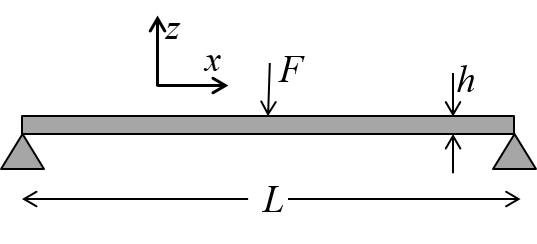
Figure-1: 3-point bending

m1={'E1':140000, 'E2':10000, 'v12':0.3, 'G12':5000}

layup = [ {'mat':m1 , 'ori': 0   , 'thi':1} , 
          {'mat':m1 , 'ori':90   , 'thi':1} ,
          {'mat':m1 , 'ori': 0   , 'thi':1} ,
          {'mat':m1 , 'ori':90   , 'thi':1} ,
          {'mat':m1 , 'ori': 0   , 'thi':1} ]

L,b,F = 200,20,100

ABD = laminateStiffnessMatrix(layup)

Db = b*(ABD[3,3]-(ABD[3,4]**2)/ABD[4,4])

deflection = (F*L**3)/(48*Db)

print(deflection,'mm')

0.7051793480852432 mm

For a single layer laminate we find that

$$\begin{equation} b \big ( D_{xx} - \frac{D_{xy}^2}{D_{yy}} \big) = E_x \frac{b h^3}{12} \tag{29} \end{equation}$$

layup = [ {'mat':m1 , 'ori': 0   , 'thi':1}  ]

b=20
ABD = laminateStiffnessMatrix(layup)
Db = b*(ABD[3,3]-(ABD[3,4]**2)/ABD[4,4])

print(Db)

I=b*(layup[0]['thi']**3)/12

print(m1['E1']*I)

233333.33333333337
233333.33333333334

Effective strength and failure envelopes

The following examples will be explored and discussed in lectures

import matlib
from laminatelib import solveLaminateLoadCase, layerResults
m1 = matlib.get('E-glass/Epoxy')
layup = [ {'mat':m1 , 'ori': 0    , 'thi':1} , 
          {'mat':m1 , 'ori': -45  , 'thi':1} ,
          {'mat':m1 , 'ori': 45   , 'thi':1} ,
          {'mat':m1 , 'ori': 90   , 'thi':1} ,
          {'mat':m1 , 'ori': 90   , 'thi':1} ,
          {'mat':m1 , 'ori': 45   , 'thi':1} ,
          {'mat':m1 , 'ori': -45  , 'thi':1} ,
          {'mat':m1 , 'ori': 0    , 'thi':1}  ]

ABD=laminateStiffnessMatrix(layup)
loads,defs=solveLaminateLoadCase(ABD, Nx=1)
h=laminateThickness(layup)
res=layerResults(layup,defs)
fE=0
for r in res:
    if r['fail']['TW']['bot']>fE:
        fE=r['fail']['TW']['bot']
print('Effective strength, sx =', 1/(fE*h),'MPa')    

Effective strength, sx = 82.12455796477958 MPa

fig,ax = plt.subplots(figsize=(8,8))
sx_0,sy_0=[],[]
sx_45,sy_45=[],[]
sx_90,sy_90=[],[]
for a in np.linspace(0,360,3600):
    Nx=np.cos(np.radians(a))
    Ny=np.sin(np.radians(a))
    loads,defs=solveLaminateLoadCase(ABD, Nx=Nx, Ny=Ny)
    res=layerResults(layup,defs)
    # 0-layers:
    fE=res[0]['fail']['TW']['bot']
    sx_0.append(Nx/(fE*h))
    sy_0.append(Ny/(fE*h))
    # +-45 layers:
    fE=res[1]['fail']['TW']['bot']
    sx_45.append(Nx/(fE*h))
    sy_45.append(Ny/(fE*h))
    # 90-layers:
    fE=res[3]['fail']['TW']['bot']
    sx_90.append(Nx/(fE*h))
    sy_90.append(Ny/(fE*h))
ax.plot(sx_0,sy_0,'--',color='blue',linewidth=1)
ax.plot(sx_45,sy_45,'--',color='green',linewidth=1)
ax.plot(sx_90,sy_90,'--',color='red',linewidth=1)
ax.scatter((0,),(0,),c='black', marker='+',s=500)
ax.set_xlabel(r'$\sigma_x$',fontsize=14)
ax.set_ylabel(r'$\sigma_y$',fontsize=14)
#ax.set_xlim(-1000,1000)
#ax.set_ylim(-1000,1000)
ax.grid(True)
plt.tight_layout()

m1['E2']=0.01*m1['E2']
m1['G12']=0.01*m1['G12']

fig,ax = plt.subplots(figsize=(8,8))
sx_0,sy_0=[],[]
sx_45,sy_45=[],[]
sx_90,sy_90=[],[]
for a in np.linspace(0,360,3600):
    Nx=np.cos(np.radians(a))
    Ny=np.sin(np.radians(a))
    loads,defs=solveLaminateLoadCase(ABD, Nx=Nx, Ny=Ny)
    res=layerResults(layup,defs)
    # 0-layers:
    fE=res[0]['fail']['TW']['bot']
    sx_0.append(Nx/(fE*h))
    sy_0.append(Ny/(fE*h))
    # +-45 layers:
    fE=res[1]['fail']['TW']['bot']
    sx_45.append(Nx/(fE*h))
    sy_45.append(Ny/(fE*h))
    # 90-layers:
    fE=res[3]['fail']['TW']['bot']
    sx_90.append(Nx/(fE*h))
    sy_90.append(Ny/(fE*h))
ax.plot(sx_0,sy_0,'--',color='blue',linewidth=1)
ax.plot(sx_45,sy_45,'--',color='green',linewidth=1)
ax.plot(sx_90,sy_90,'--',color='red',linewidth=1)
ax.scatter((0,),(0,),c='black', marker='+',s=500)
ax.set_xlabel(r'$\sigma_x$',fontsize=14)
ax.set_ylabel(r'$\sigma_y$',fontsize=14)
ax.grid(True)
plt.tight_layout()

fig,ax = plt.subplots(figsize=(8,8))
ax.plot(sx_0,sy_0,'--',color='blue',linewidth=1)
ax.plot(sx_45,sy_45,'--',color='green',linewidth=1)
ax.plot(sx_90,sy_90,'--',color='red',linewidth=1)
ax.scatter((0,),(0,),c='black', marker='+',s=500)
ax.set_xlabel(r'$\sigma_x$',fontsize=14)
ax.set_ylabel(r'$\sigma_y$',fontsize=14)
ax.set_xlim(-3000,3000)
ax.set_ylim(-3000,3000)
ax.grid(True)
plt.tight_layout()

Disclaimer:This site is about polymer composites, designed for educational purposes. Consumption and use of any sort & kind is solely at your own risk.
Fair use: I spent some time making all the pages, and even the figures and illustrations are my own creations. Obviously, you may steal whatever you find useful here, but please show decency and give some acknowledgment if or when copying. Thanks! Contact me: nils.p.vedvik@ntnu.no www.ntnu.edu/employees/nils.p.vedvik

Copyright 2021, All right reserved, I guess.