Failure criteria
A failure criterion is fundamentally a set of rules, functions or other expressions of logic that judges if a given state of loading will cause failure or not. For example, the Maximum stress criterion can be stated simply as: failure is predicted if any of the stress components exceeds the corresponding strengths.
Maximum stress criterion
The Maximum stress failure criterion makes a simple asessment where each stress component is compared to the corresponding strength. The criterion predicts failure if one of the following six conditions is False:
\begin{equation} \begin{aligned} & -X_C < \sigma_1 < X_T && -Y_C < \sigma_2 < Y_T && -Z_C < \sigma_3 < Z_T && \mid\tau_{12}\mid <S_{12} && \mid\tau_{13}\mid < S_{13} && \mid\tau_{23}\mid < S_{23} \end{aligned} \tag{1} \end{equation}The criterion can alternatively be formulated using a max function:
\begin{equation} f = \text{max}\Big( -\frac{\sigma_1}{X_C}, \frac{\sigma_1}{X_T}, -\frac{\sigma_2}{Y_C}, \frac{\sigma_2}{Y_T}, -\frac{\sigma_3}{Z_C}, \frac{\sigma_3}{Z_T}, \frac{|\tau_{12}|}{S_{12}}, \frac{|\tau_{13}|}{S_{13}}, \frac{|\tau_{23}|}{S_{23}}\Big) \tag{2} \end{equation}where failure is predicted when $f \geq 1$.
The stress exposure factor is obtained by multiplying the load proportionality factor $R$ to each stress components and equating the result to unity:
\begin{equation}\text{max}\Big( -\frac{R\sigma_1}{X_C}, \frac{R\sigma_1}{X_T}, -\frac{R\sigma_2}{Y_C}, \frac{R\sigma_2}{Y_T}, -\frac{R\sigma_3}{Z_C}, \frac{R\sigma_3}{Z_T}, \frac{R|\tau_{12}|}{S_{12}}, \frac{R|\tau_{13}|}{S_{13}}, \frac{R|\tau_{23}|}{S_{23}}\Big) = 1 \tag{3} \end{equation}such that
\begin{equation} f_E = \frac{1}{R} = \text{max}\Big( -\frac{\sigma_1}{X_C}, \frac{\sigma_1}{X_T}, -\frac{\sigma_2}{Y_C}, \frac{\sigma_2}{Y_T}, -\frac{\sigma_3}{Z_C}, \frac{\sigma_3}{Z_T}, \frac{|\tau_{12}|}{S_{12}}, \frac{|\tau_{13}|}{S_{13}}, \frac{|\tau_{23}|}{S_{23}}\Big) \tag{4} \end{equation}Implementation:
The following function returns the stress exposure factor $f_E$ for a stress state s and material m:
def fE_maxstress(s,m):
    # Using local varibles for easier coding and readability..
    s1,s2,s3,s23,s13,s12=s[0],s[1],s[2],s[3],s[4],s[5]
    XT,YT,ZT,XC,YC,ZC,S12,S13,S23 = m['XT'], m['YT'], m['ZT'], m['XC'], m['YC'], m['ZC'], m['S12'], m['S13'], m['S23']
    fE=max(s1/XT,-s1/XC,s2/YT,-s2/YC,s3/ZT,-s3/ZC,abs(s12/S12),abs(s13/S13),abs(s23/S23))
    return fE
Example:
import matlib
m1=matlib.get('Carbon/Epoxy(a)')
stressCases = (150, 0, 0, 0, 0, 0) , (-120,-60,0,0,0,0) , (1000,60,0,0,0,0) , (0,0,0,0,0,150)

for s in stressCases:
    fE=fE_maxstress(s,m1)
    print('fE =',fE,'when stress=',s)
Failure envelope in the $\sigma_1$ - $\sigma_2$ -plane:
import matplotlib.pyplot as plt
%matplotlib inline

#Data points for the rectangle in the s1-s2 plane
s1=(m1['XT'],-m1['XC'],-m1['XC'],m1['XT'],m1['XT'])
s2=(m1['YT'],m1['YT'],-m1['YC'],-m1['YC'],m1['YT'])
fig,ax = plt.subplots(figsize=(8,4))
ax.plot(s1,s2,'--',color='blue',linewidth=1)

#Origo
ax.plot((0,),(0,),'+',color='black',markersize=50)

#Adding some stress states

s1a, s2a = -600, -50
s1b, s2b = 180, 0
s1c, s2c = 1000, 60

ax.scatter((s1a,s1b,s1c),(s2a,s2b,s2c),color='red')
fE1=fE_maxstress((s1a,s2a,0,0,0,0),m1)
fE2=fE_maxstress((s1b,s2b,0,0,0,0),m1)
fE3=fE_maxstress((s1c,s2c,0,0,0,0),m1)
ax.text(s1a,s2a,'  '+r'$f_E=$'+str(fE1),fontsize=14)
ax.text(s1b,s2b,'  '+r'$f_E=$'+str(fE2),fontsize=14)
ax.text(s1c,s2c,'  '+r'$f_E=$'+str(fE3),fontsize=14)
ax.set_xlabel(r'$\sigma_1$',fontsize=14)
ax.set_ylabel(r'$\sigma_2$',fontsize=14)
ax.grid(True)
plt.tight_layout()

Maximum stress envelope in the $\sigma_1$ - $\sigma_2$ -plane plane can be constructed using a more generic method where we sweep through $\theta=0...360^{\circ}$ where $\sigma_1=\cos(\theta)$ and $\sigma_2=\sin(\theta)$. This method can be utilized for most failure criteria.
fig,ax = plt.subplots(figsize=(8,4))

# empty list of the stresses in the 1-2 plane:
s1,s2=[],[]

# sweeping 360 degrees using 10 points per degrees:

import numpy as np

for a in np.linspace(0,360,3600):
    s1i=np.cos(np.radians(a))
    s2i=np.sin(np.radians(a))
    fe=fE_maxstress((s1i,s2i,0,0,0,0),m1)
    # then scaling by the load-proportionality ratio (1/fE):
    s1.append(s1i/fe)
    s2.append(s2i/fe)

ax.plot(s1,s2,'--',color='blue',linewidth=1)

ax.plot((0,),(0,),'+',color='black',markersize=50)

ax.set_xlabel(r'$\sigma_1$',fontsize=14)
ax.set_ylabel(r'$\sigma_2$',fontsize=14)

ax.grid(True)

plt.tight_layout()

Maximum strain criterion
The Maximum strain criterion follows the same principle as the Maximum stress criterion, where strain components are compared to corresponding failure strains. When assuming linear relations between stresses and strains, the criteria can be expressed as
\begin{equation} f = max\Big( -\frac{\varepsilon_1}{X_C/E_1}, \frac{\varepsilon_1}{X_T/E_1}, -\frac{\varepsilon_2}{Y_C/E_2}, \frac{\varepsilon_2}{Y_T/E_2}, -\frac{\varepsilon_3}{Z_C/E_3}, \frac{\varepsilon_3}{Z_T/E_3}, \frac{|\gamma_{12}|}{S_{12}/G_{12}}, \frac{|\gamma_{13}|}{S_{13}/G_{13}}, \frac{|\gamma_{23}|}{S_{23}/G_{23}}\Big) \tag{5}\end{equation}A function for the stress exposure factor $f_E$:
def fE_maxstrain(s,m):
    s1,s2,s3,s23,s13,s12=s[0],s[1],s[2],s[3],s[4],s[5]
    XT,YT,ZT,XC,YC,ZC,S12,S13,S23 = m['XT'],m['YT'],m['ZT'],m['XC'],m['YC'],m['ZC'],m['S12'],m['S13'],m['S23']
    E1,E2,E3,v12,v13,v23,G12,G13,G23=m['E1'],m['E2'],m['E3'],m['v12'],m['v13'],m['v23'],m['G12'],m['G13'],m['G23']
    e1=   (1/E1)*s1 + (-v12/E1)*s2 + (-v13/E1)*s3
    e2=(-v12/E1)*s1 +    (1/E2)*s2 + (-v23/E2)*s3
    e3=(-v13/E1)*s1 + (-v23/E2)*s2 +    (1/E3)*s3
    e23,e13,e12 = s23/G23, s13/G13, s12/G12
    f=max( e1/(XT/E1),-e1/(XC/E1),e2/(YT/E2),-e2/(YC/E2),e3/(ZT/E3),-e3/(ZC/E3),
           abs(e12/(S12/G12)),abs(e13/(S13/G13)),abs(e23/(S23/G23)) )
    return f
Example:
import matlib
m1=matlib.get('Carbon/Epoxy(a)')
stress1, stress2, stress3, stress4 = (150, 0, 0, 0, 0, 0) , (-120,-60,0,0,0,0) , (1000,60,0,0,0,0) , (0,0,0,0,0,150)
print()
fE1=fE_maxstrain(stress1,m1)
fE2=fE_maxstrain(stress2,m1)
fE3=fE_maxstrain(stress3,m1)
fE4=fE_maxstrain(stress4,m1)
print('Exposure factor for case stress1: ',fE1)
print('Exposure factor for case stress2: ',fE2)
print('Exposure factor for case stress3: ',fE3)
print('Exposure factor for case stress4: ',fE4)
Failure envelope, $\sigma_1$ versus $\sigma_2$:
import matplotlib.pyplot as plt
%matplotlib inline
fig,ax = plt.subplots(figsize=(8,4))

# empty list of normal stresses in the 1-2 plane:
s1,s2=[],[]

# sweeping 0-3600 points

from math import cos,sin,radians

for a in range(0,3600):
    s1i=cos(radians(a/10))
    s2i=sin(radians(a/10))
    fe=fE_maxstrain((s1i,s2i,0,0,0,0),m1)
    # then scaling by the load-proportionality ratio (1/fE):
    s1.append(s1i/fe)
    s2.append(s2i/fe)

ax.plot(s1,s2,'--',color='blue',linewidth=1)
#Making axes through the origo:
ax.plot((0,),(0,),'+',color='black',markersize=50)

ax.set_xlabel(r'$\sigma_1$',fontsize=14)
ax.set_ylabel(r'$\sigma_2$',fontsize=14)

ax.grid(True)

plt.tight_layout()

Failure envelope, $\sigma_2$ versus $\sigma_3$:
fig,ax = plt.subplots(figsize=(6,6))
# empty list of normal stresses in the 1-2 plane:
s2,s3=[],[]

# sweeping 0-3600 points:

from math import cos,sin,radians

for a in range(0,3600):
    s2i=cos(radians(a/10))
    s3i=sin(radians(a/10))
    fe=fE_maxstrain((0,s2i,s3i,0,0,0),m1)
    # then scaling by the load-proportionality ratio (1/fE):
    s2.append(s2i/fe)
    s3.append(s3i/fe)

ax.plot(s2,s3,'--',color='blue',label='Maximum strain',linewidth=1)
ax.plot((0,),(0,),'+',color='black',markersize=50)
ax.legend(loc='best')

ax.set_xlabel(r'$\sigma_2$',fontsize=14)
ax.set_ylabel(r'$\sigma_3$',fontsize=14)

ax.grid(True)

plt.tight_layout()

The 3-dimensional maximum strain criterion produces a few highly inconsistent results, one of them shows up in the last envelope where apparantly a basic strength parameter has changed... To be discussed in lectures
Tsai-Wu criterion
The Tsai-Wu failure criterion is a specialization of the general quadratic failure criterion and is expressed in the form
\begin{equation} \begin{split} f = & F_1\sigma_1 + F_2\sigma_2 + F_3\sigma_3 + F_{11}\sigma_1^2 + F_{22}\sigma_2^2 + F_{33}\sigma_3^2+ \\ & F_{44}\tau_{23}^2 + F_{55}\tau_{13}^2 + F_{66}\tau_{12}^2 + 2F_{23}\sigma_2\sigma_3 + 2F_{13}\sigma_1\sigma_3 + 2F_{12}\sigma_1\sigma_2 \end{split} \tag{6} \end{equation}where failure is predicted when $f\geq1$
The coefficients are expressed by the basic strength parameters,
\begin{equation} \begin{aligned} &F_1=\frac{1}{X_T}-\frac{1}{X_C}, \quad F_2=\frac{1}{Y_T}-\frac{1}{Y_C}, \quad F_3=\frac{1}{Z_T}-\frac{1}{Z_C} \\ &F_{11}=\frac{1}{X_T X_C}, \quad F_{22}=\frac{1}{Y_TY_C}, \quad F_{33}=\frac{1}{Z_TZ_C} \\ &F_{44}=\frac{1}{S_{23}^2}, \quad F_{55}=\frac{1}{S_{13}^2}, \quad F_{66}=\frac{1}{S_{12}^2} \\ &F_{23}=f_{23}\sqrt{F_{22}F_{33}}, \quad F_{13}=f_{13}\sqrt{F_{11}F_{33}}, \quad F_{12}=f_{12}\sqrt{F_{11}F_{22}} \end{aligned} \tag{7} \end{equation}where $f_{12},f_{13},f_{23}$ are experimentally determined interaction coefficients.
Solving the quadratic equation:
\begin{equation} \begin{split} & (F_1\sigma_1 + F_2\sigma_2 + F_3\sigma_3)R + \\ &(F_{11}\sigma_1^2 + F_{22}\sigma_2^2 + F_{33}\sigma_3^2 + F_{44}\tau_{23}^2 + F_{55}\tau_{13}^2 + F_{66}\tau_{12}^2 + 2F_{23}\sigma_2\sigma_3 + 2F_{13}\sigma_1\sigma_3 + 2F_{12}\sigma_1\sigma_2)R^2 = 1 \end{split} \tag{8} \end{equation}Such that
\begin{equation} \begin{aligned} &a=F_{11}\sigma_1^2 + F_{22}\sigma_2^2 + F_{33}\sigma_3^2 + F_{44}\tau_{23}^2 + F_{55}\tau_{13}^2 + F_{66}\tau_{12}^2 + 2F_{23}\sigma_2\sigma_3 + 2F_{13}\sigma_1\sigma_3 + 2F_{12}\sigma_1\sigma_2 \\ &b= F_1\sigma_1 + F_2\sigma_2 + F_3\sigma_3 \\ &c=-1 \end{aligned} \tag{9} \end{equation}and
\begin{equation} R=\frac{-b+\sqrt{b^2 -4ac}}{2a} \tag{10} \end{equation}Observe that the parameter $a$ can be zero. In such a case the $R$ will be undefined. In those cases we just return zero as written in this code:
def fE_tsaiwu(s,m):
    s1,s2,s3,s23,s13,s12=s[0],s[1],s[2],s[3],s[4],s[5]
    XT,YT,ZT,XC,YC,ZC,S12,S13,S23 = m['XT'], m['YT'], m['ZT'], m['XC'], m['YC'], m['ZC'], m['S12'], m['S13'], m['S23']
    f12, f13, f23 = m['f12'], m['f13'], m['f23']
    F1,  F2,  F3  = (1/XT)-(1/XC) , (1/YT)-(1/YC) , (1/ZT)-(1/ZC)
    F11, F22, F33 =     1/(XT*XC) ,     1/(YT*YC) ,     1/(ZT*ZC)
    F44, F55, F66 =    1/(S23**2) ,    1/(S13**2) ,     1/(S12**2)
    F12 = f12*(F11*F22)**0.5
    F13 = f13*(F11*F33)**0.5
    F23 = f23*(F22*F33)**0.5
    a=F11*(s1**2) + F22*(s2**2) + F33*(s3**2)+ 2*(F12*s1*s2 + F13*s1*s3 + F23*s2*s3)+\
    F44*(s23**2) + F55*(s13**2) + F66*(s12**2)
    if a==0:
        return 0
    b=F1*s1 + F2*s2 +F3*s3
    c=-1
    R=(-b+(b**2-4*a*c)**0.5)/(2*a)
    fE=1/R
    return fE
Example
import matlib
m1=matlib.get('Carbon/Epoxy(a)')

stressCases = (150, 0, 0, 0, 0, 0) , (-120,-60,0,0,0,0) , (1000,60,0,0,0,0) , (0,0,0,0,0,150)

for s in stressCases:
    fE=fE_tsaiwu(s,m1)
    print(fE)
Failure envelope, $\sigma_2$ versus $\sigma_1$:
import matplotlib.pyplot as plt
import numpy as np
%matplotlib inline

fig,ax = plt.subplots(figsize=(8,4))
s1,s2=[],[]

from math import cos,sin,radians
for a in np.linspace(0,360,3600):
    s1i=cos(radians(a))
    s2i=sin(radians(a))
    fe=fE_tsaiwu((s1i,s2i,0,0,0,0),m1)
    s1.append(s1i/fe)
    s2.append(s2i/fe)

ax.plot(s1,s2,'-',color='blue',label='Tsai-Wu',linewidth=1)
ax.plot((0,),(0,),'+',color='black',markersize=50)
ax.legend(loc='best')

ax.set_xlabel(r'$\sigma_1$',fontsize=14)
ax.set_ylabel(r'$\sigma_2$',fontsize=14)
ax.grid(True)

plt.tight_layout()

Failure envelope, $\sigma_2$ versus $\sigma_1$ for constant nonzero values of $\tau_{12}$:
Terms of a, b in equtions (4) containing $\tau_{12}$ are now constants and therefor terms of the constant c:
\begin{equation} \begin{aligned} & a=F_{11}\sigma_1^2 + F_{22}\sigma_2^2 + F_{33}\sigma_3^2 + F_{44}\tau_{23}^2 + F_{55}\tau_{13}^2 + 2F_{23}\sigma_2\sigma_3 + 2F_{13}\sigma_1\sigma_3 + 2F_{12}\sigma_1\sigma_2 \\ &b= F_1\sigma_1 + F_2\sigma_2 + F_3\sigma_3 \\ &c=-1 + F_{66}\tau_{12}^2 \end{aligned} \tag{11} \end{equation}Modified function for the specific case:
def fE_tsaiwu_const_s12(s,m):
    s1,s2,s3,s23,s13,s12=s[0],s[1],s[2],s[3],s[4],s[5]
    XT,YT,ZT,XC,YC,ZC,S12,S13,S23 = m['XT'], m['YT'], m['ZT'], m['XC'], m['YC'], m['ZC'], m['S12'], m['S13'], m['S23']
    f12, f13, f23 = m['f12'], m['f13'], m['f23']
    F1,  F2,  F3  = (1/XT)-(1/XC) , (1/YT)-(1/YC) , (1/ZT)-(1/ZC)
    F11, F22, F33 =     1/(XT*XC) ,     1/(YT*YC) ,     1/(ZT*ZC)
    F44, F55, F66 =    1/(S23**2) ,    1/(S13**2) ,     1/(S12**2)
    F12 = f12*(F11*F22)**0.5
    F13 = f13*(F11*F33)**0.5
    F23 = f23*(F22*F33)**0.5
    a=F11*(s1**2) + F22*(s2**2) + F33*(s3**2)+ 2*(F12*s1*s2 + F13*s1*s3 + F23*s2*s3)+\
    F44*(s23**2) + F55*(s13**2)
    if a==0:
        return 0
    b=F1*s1 + F2*s2 +F3*s3
    c=-1 + F66*(s12**2)
    R=(-b+(b**2-4*a*c)**0.5)/(2*a)
    fE=1/R
    return fE
Multiple failure envelopes:
fig,ax = plt.subplots(figsize=(12,8))
s1a,s2a,s1b,s2b,s1c,s2c,s1d,s2d,s1e,s2e=[],[],[],[],[],[],[],[],[],[]

from math import cos,sin,radians
for a in np.linspace(0,360,3600):
    s1i=cos(radians(a))
    s2i=sin(radians(a))
    fea=fE_tsaiwu_const_s12((s1i,s2i,0,0,0,0),m1)
    feb=fE_tsaiwu_const_s12((s1i,s2i,0,0,0,20),m1)
    fec=fE_tsaiwu_const_s12((s1i,s2i,0,0,0,40),m1)
    fed=fE_tsaiwu_const_s12((s1i,s2i,0,0,0,50),m1)
    fee=fE_tsaiwu_const_s12((s1i,s2i,0,0,0,60),m1)
    s1a.append(s1i/fea)
    s2a.append(s2i/fea)
    s1b.append(s1i/feb)
    s2b.append(s2i/feb)
    s1c.append(s1i/fec)
    s2c.append(s2i/fec)
    s1d.append(s1i/fed)
    s2d.append(s2i/fed)
    s1e.append(s1i/fee)
    s2e.append(s2i/fee)

ax.plot(s1a,s2a,'-',color='blue',label=r'Tsai-Wu, $\tau_{12}$=0',linewidth=1)
ax.plot(s1b,s2b,'-',color='red',label=r'Tsai-Wu, $\tau_{12}$=20',linewidth=1)
ax.plot(s1c,s2c,'-',color='green',label=r'Tsai-Wu, $\tau_{12}$=40',linewidth=1)
ax.plot(s1d,s2d,'-',color='orange',label=r'Tsai-Wu, $\tau_{12}$=50',linewidth=1)
ax.plot(s1e,s2e,'-',color='cyan',label=r'Tsai-Wu, $\tau_{12}$=60',linewidth=1)
ax.plot((0,),(0,),'+',color='black',markersize=50)
ax.legend(loc='best')

ax.set_xlabel(r'$\sigma_1$',fontsize=14)
ax.set_ylabel(r'$\sigma_2$',fontsize=14)
ax.grid(True)

plt.tight_layout()

Inconsistency of the criterion
Imagine now that we, for whatever reason, find it reasonable to use a lower value of the transverse tensile strength $X_T$:
m1['YT']=25
Then, construct the failure envelopes for both cases:
fig,ax = plt.subplots(figsize=(8,4))
s1b,s2b=[],[]

from math import cos,sin,radians
for a in np.linspace(0,360,3600):
    s1i=cos(radians(a))
    s2i=sin(radians(a))
    fe=fE_tsaiwu((s1i,s2i,0,0,0,0),m1)
    # then scaling by the load-proportionality ratio (1/fE):
    s1b.append(s1i/fe)
    s2b.append(s2i/fe)

ax.plot(s1,s2,'-',color='blue',label=r'Tsai-Wu, $Y_T$=50',linewidth=1)
ax.plot(s1b,s2b,'-',color='red',label=r'Tsai-Wu, $Y_T$=25',linewidth=1)
ax.plot((0,),(0,),'+',color='black',markersize=50)
ax.legend(loc='best')

ax.set_xlabel(r'$\sigma_1$',fontsize=14)
ax.set_ylabel(r'$\sigma_2$',fontsize=14)
#ax.set_xticks([0])
#ax.set_yticks([0])
ax.grid(True)

plt.tight_layout()

So, reduced transverse tensile strength implies improved capacity in compression-compression?
To be discussed in lectures
Hashin criterion
The 3D Hashin Criterion (1980) divides the mechanisms of failure of UD fiber composite materials intwo two groups: Fiber Failure (FF) and Inter Fiber Failure (IFF). Both of these are divided into tensile mode and compressive mode:
Fiber failure (FF) when $\sigma_1 > 0:$
\begin{equation} \Big( \frac{\sigma_1}{X_T} \Big)^2 + \frac{1}{S_{12}^2}\Big( \tau_{12}^2 + \tau_{13}^2 \Big) = 1 \tag{12} \end{equation}Fiber failure (FF) when $\sigma_1 \le 0:$
\begin{equation} -\frac{\sigma_1}{X_C} = 1 \tag{13} \end{equation}Inter fiber failure (IFF) when $(\sigma_2 + \sigma_3) \ge 0:$
\begin{equation} \frac{1}{Y_T^2}(\sigma_2+\sigma_3)^2 + \frac{1}{S_{23}^2}(\tau_{23}^2-\sigma_2 \sigma_3 ) + \frac{1}{S_{12}^2}(\tau_{12}^2+\tau_{13}^2 \ ) = 1 \tag{14} \end{equation}Inter fiber failure (IFF) when $(\sigma_2 + \sigma_3) < 0:$
\begin{equation} \frac{1}{4S_{23}^2} (\sigma_2+\sigma_3)^2 + \frac{1}{S_{23}^2}(\tau_{23}^2-\sigma_2 \sigma_3 ) + \frac{1}{S_{12}^2}(\tau_{12}^2+\tau_{13}^2 \ ) + \frac{1}{Y_C}\Big( \frac{Y_C^2}{4S_{23}^2} - 1 \Big)(\sigma_2+\sigma_3) = 1 \tag{15} \end{equation}Implementation
def fE_hashin(s,m):
    s1,s2,s3,s23,s13,s12=s[0],s[1],s[2],s[3],s[4],s[5]
    XT,YT,ZT,XC,YC,ZC,S12,S13,S23 = m['XT'], m['YT'], m['ZT'], m['XC'], m['YC'], m['ZC'], m['S12'], m['S13'], m['S23']
    if s1>0:
        R = ( 1/( (s1/XT)**2 + (1/S12**2)*(s12**2 + s13**2) ) )**0.5
        fE_FF=1/R
    if s1<=0:
        fE_FF=-s1/XC
    if (s2+s3)>=0:
        temp=( (1/YT**2)*(s2+s3)**2+(1/S23**2)*(s23**2-s2*s3)+(1/S12**2)*(s12**2+s13**2) )
        if temp==0:
            fE_IFF = 0
        else:
            R = (1/temp)**0.5
            fE_IFF = 1/R
    if (s2+s3)<0:
        b = (1/YC)*((YC/(2*S23))**2-1)*(s2+s3)
        a = (1/(4*S23**2))*(s2+s3)**2+(1/S23**2)*(s23**2-s2*s3)+(1/S12**2)*(s12**2+s13**2)
        if a==0:
            fE_IFF = 0.0
        else:
            c=-1
            R=(-b+(b**2-4*a*c)**0.5)/(2*a)
            fE_IFF = 1/R
    return fE_FF, fE_IFF
Example
import matlib
m1=matlib.get('Carbon/Epoxy(a)')

s = (1200, -20, 10, 30, 0, 0)

ff,iff = fE_hashin(s,m1)
print('Exposure factors for FF and IFF:')
print(ff,'and', iff)
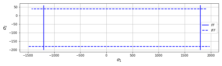
Failure envelopes, $\sigma_2$ versus $\sigma_1$
Fiber failure (FF) is reduced to a simple maximum stress criterion when only $\sigma_2$ and $\sigma_1$ are present:
When $\sigma_1 > 0:$
\begin{equation} \Big( \frac{\sigma_1}{X_T} \Big)^2 = 1 \Rightarrow \frac{\sigma_1}{X_T}=1 \end{equation}When $\sigma_1 \le 0:$
\begin{equation} -\frac{\sigma_1}{X_C} = 1 \end{equation}Inter fiber failure (IFF) when $(\sigma_2 + \sigma_3) \ge 0$ is also just a maximum stress criterion;
\begin{equation} \Big(\frac{\sigma_2}{Y_T}\Big)^2 = 1 \Rightarrow \frac{\sigma_2}{Y_T}=1 \end{equation}Inter fiber failure (IFF) when $(\sigma_2 + \sigma_3) < 0:$
\begin{equation} \frac{\sigma_2^2}{4S_{23}^2} + \frac{1}{Y_C}\Big( \frac{Y_C^2}{4S_{23}^2} - 1 \Big)\sigma_2 = 1 \Rightarrow \end{equation}\begin{equation} \frac{Y_C^2}{4S_{23}^2} - \frac{1}{Y_C}\Big( \frac{Y_C^2}{4S_{23}^2} - 1 \Big)Y_C = 1 \quad \text{when} \quad \sigma_2 = -Y_C \end{equation}Failure envelope for the material Carbon/Epoxy(a):
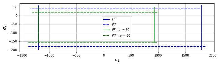
A non-zero shear stress $\tau_{12}$ will reduce the envelope for all modes but the compressive fiber failure:
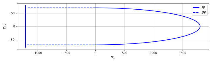
Failure envelopes, $\tau_{12}$ versus $\sigma_1$:
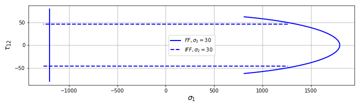
Failure envelopes, $\tau_{12}$ versus $\sigma_2$
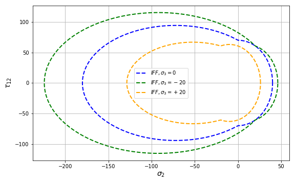
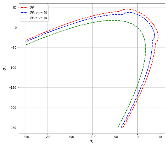
Failure envelopes, $\sigma_3$ versus $\sigma_2$
Comparing failure criteria
Previously implemented functions:
from compositelib import fE_maxstress, fE_maxstrain, fE_tsaiwu, fE_hashin
Material properties for the examples:
import matlib
m1=matlib.get('Carbon/Epoxy(a)')
import matplotlib.pyplot as plt
%matplotlib inline
fig,ax = plt.subplots(figsize=(8,4))
# empty list of normal stresses in the 1-2 plane:
s1_MS,s2_MS=[],[]  # maximum stress
s1_ME,s2_ME=[],[]  # maximum strain
s1_TW,s2_TW=[],[]  # tsai-wu

from math import cos,sin,radians
for a in range(0,3600):
    s1i=cos(radians(a/10))
    s2i=sin(radians(a/10))
    feMS=fE_maxstress((s1i,s2i,0,0,0,0),m1)
    feME=fE_maxstrain((s1i,s2i,0,0,0,0),m1)
    feTW=fE_tsaiwu((s1i,s2i,0,0,0,0),m1)
    # then scaling by the load-proportionality ratio (1/fE):
    s1_MS.append(s1i/feMS)
    s2_MS.append(s2i/feMS)
    s1_ME.append(s1i/feME)
    s2_ME.append(s2i/feME)
    s1_TW.append(s1i/feTW)
    s2_TW.append(s2i/feTW)

ax.plot(s1_MS,s2_MS,'--',color='black',label='Max Stress',linewidth=1)
ax.plot(s1_ME,s2_ME,'--',color='blue',label='Max Strain',linewidth=1)
ax.plot(s1_TW,s2_TW,'--',color='green',label='Tsai-Wu',linewidth=1)

ax.plot((0,),(0,),'+',color='black',markersize=50)
ax.grid(True)
ax.legend(loc='best')

ax.set_xlabel(r'$\sigma_1$',fontsize=14)
ax.set_ylabel(r'$\sigma_2$',fontsize=14)

plt.tight_layout()

import matplotlib.pyplot as plt
%matplotlib inline
fig,ax = plt.subplots(figsize=(6,6))
s2_MS,s3_MS=[],[]
s2_ME,s3_ME=[],[]
s2_TW,s3_TW=[],[]
s2_HH,s3_HH=[],[]
from math import cos,sin,radians
for a in range(0,3600):
    s2i=cos(radians(a/10))
    s3i=sin(radians(a/10))
    feMS=fE_maxstress((0,s2i,s3i,0,0,0),m1)
    feME=fE_maxstrain((0,s2i,s3i,0,0,0),m1)
    feTW=fE_tsaiwu((0,s2i,s3i,0,0,0),m1)
    feHH=fE_hashin((0,s2i,s3i,0,0,0),m1)[1]
    # then scaling by the load-proportionality ratio (1/fE):
    s2_MS.append(s2i/feMS)
    s3_MS.append(s3i/feMS)
    s2_ME.append(s2i/feME)
    s3_ME.append(s3i/feME)
    s2_TW.append(s2i/feTW)
    s3_TW.append(s3i/feTW)
    if feHH>0:
        s2_HH.append(s2i/feHH)
        s3_HH.append(s3i/feHH)

ax.plot(s2_MS,s3_MS,'--',color='black',label='Max Stress',linewidth=1)
ax.plot(s2_ME,s3_ME,'--',color='blue',label='Max Strain',linewidth=1)
ax.plot(s2_TW,s3_TW,'--',color='green',label='Tsai-Wu',linewidth=1)
ax.plot(s2_HH,s3_HH,'--',color='orange',label='Hashin',linewidth=1)

ax.plot((0,),(0,),'+',color='black',markersize=50)
ax.grid(True)
ax.legend(loc='best')

ax.set_xlabel(r'$\sigma_2$',fontsize=14)
ax.set_ylabel(r'$\sigma_3$',fontsize=14)

ax.set_xlim(-300,100)
ax.set_ylim(-300,100)

plt.tight_layout()

Plane stress failure criteria
The Maximum stress failure criterion for plane stress case is derived by simply eliminating the stress-terms not being relevant in the 3D expression:
\begin{equation} f_E = max\Big[ -\frac{\sigma_1}{X_C}, \frac{\sigma_1}{X_T}, -\frac{\sigma_2}{Y_C}, \frac{\sigma_2}{Y_T}, \frac{|\tau_{12}|}{S_{12}}\Big] \tag{16} \end{equation}def fE2DMS(s,m):
s1,s2,s12=s[0],s[1],s[2]
XT,YT,XC,YC,S12 = m['XT'], m['YT'], m['XC'], m['YC'], m['S12']
f=max(s1/XT,-s1/XC,s2/YT,-s2/YC,abs(s12/S12))
return f
The Maximum strain criterion reduced to the 2D case neglects the out-of plane components of strains:
\begin{equation} f_E = max\Big[ -\frac{\epsilon_1}{X_C/E_1}, \frac{\epsilon_1}{X_T/E_1}, -\frac{\epsilon_2}{Y_C/E_2}, \frac{\epsilon_2}{Y_T/E_2}, \frac{|\gamma_{12}|}{S_{12}/G_{12}}\Big] \tag{17} \end{equation}def fE2DME(s,m):
s1,s2,s12=s[0],s[1],s[2]
XT,YT,XC,YC,S12 = m['XT'],m['YT'],m['XC'],m['YC'],m['S12']
E1,E2,v12,G12=m['E1'],m['E2'],m['v12'],m['G12']
e1= (1/E1)*s1 + (-v12/E1)*s2
e2=(-v12/E1)*s1 + (1/E2)*s2
e12 = s12/G12
f=max( e1/(XT/E1),-e1/(XC/E1),e2/(YT/E2),-e2/(YC/E2),abs(e12/(S12/G12)) )
return f
Tsai-Wu for plane stress is simplified to
\begin{equation} f = F_1\sigma_1+F_2\sigma_2+F_{11}\sigma_1^2+F_{22}\sigma_2^2+F_{66}\tau_{12}^2+2F_{12}\sigma_1\sigma_2 \tag{18} \end{equation}where failure is predicted when $f\geq1$
The coefficients are expressed by the basic strength parameters: \begin{equation} \begin{aligned} &F_1=\frac{1}{X_T}-\frac{1}{X_C} && F_2=\frac{1}{Y_T}-\frac{1}{Y_C} \\ &F_{11}=\frac{1}{X_TX_C} && F_{22}=\frac{1}{Y_TY_C} \\ &F_{66}=\frac{1}{S_{12}^2} && F_{12}=f_{12}\sqrt{F_{11}F_{22}} \end{aligned} \tag{19} \end{equation}
Solving the quadratic equation:
\begin{equation} (F_1\sigma_1+F_2\sigma_2+F_3\sigma_3)R+(F_{11}\sigma_1^2+F_{22}\sigma_2^2+F_{66}\tau_{12}^2+2 F_{12}\sigma_1\sigma_2)R^2=1 \tag{20} \end{equation}Such that
\begin{equation} \begin{aligned} &a=F_{11}\sigma_1^2+F_{22}\sigma_2^2+F_{66}\tau_{12}^2+2 F_{12}\sigma_1\sigma_2 \\ &b= F_1\sigma_1+F_2\sigma_2 \\ &c=-1 \end{aligned} \tag{21} \end{equation}and
\begin{equation} R=\frac{-b+\sqrt{b^2 -4ac}}{2a} \tag{22} \end{equation}Observe that the paramtere $a$ can be zero. In such a case the $R$ will be undefined. In those cases we just return zero as written in the code:
def fE2DTW(s,m):
    s1,s2,s12=s[0],s[1],s[2]
    XT,YT,XC,YC,S12,f12 = m['XT'], m['YT'], m['XC'], m['YC'], m['S12'], m['f12']
    F1,  F2  = (1/XT)-(1/XC) , (1/YT)-(1/YC)
    F11, F22 =  1/(XT*XC) , 1/(YT*YC)
    F66 = 1/(S12**2)
    F12 = f12*(F11*F22)**0.5
    a=F11*s1**2 + F22*s2**2 + 2*F12*s1*s2 + F66*s12**2
    b=F1*s1 + F2*s2
    c=-1
    if a==0:
        return 0.0
    R=(-b+(b**2-4*a*c)**0.5)/(2*a)
    fE=1/R
    return fE
Hashin for plane stress:
Fiber failure (FF) when $\sigma_1 > 0:$
\begin{equation} \Big( \frac{\sigma_1}{X_T} \Big)^2 + \Big( \frac{\tau_{12}}{S_{12}}\Big)^2 = 1 \tag{23} \end{equation}Fiber failure (FF) when $\sigma_1 \le 0:$
\begin{equation} -\frac{\sigma_1}{X_C} = 1 \tag{24} \end{equation}Inter fiber failure (IFF) when $\sigma_2 \ge 0:$
\begin{equation} \Big(\frac{\sigma_2}{Y_T}\Big)^2 + \Big( \frac{\tau_{12}}{S_{12}^2}\Big)^2 = 1 \tag{25} \end{equation}Inter fiber failure (IFF) when $(\sigma_2 + \sigma_3) < 0:$
\begin{equation} \Big(\frac{\sigma_2}{2S_{23}}\Big)^2 + \Big(\frac{\tau_{12}}{S_{12}^2}\Big)^2 + \frac{\sigma_2}{Y_C}\Big( \frac{Y_C^2}{4S_{23}^2} - 1 \Big) = 1 \tag{26} \end{equation}def fE2DHN(s,m):
s1,s2,s12=s[0],s[1],s[2]
XT,YT,XC,YC,S12,S23 = m['XT'], m['YT'], m['XC'], m['YC'], m['S12'], m['S23']
#FF
if s1>0:
a=(s1/XT)**2 + 0*(s12/S12)**2
R=(1/a)**0.5
f_FF=1/R
if s1<0:
f_FF=-s1/XC
if s1==0:
f_FF=0.0
#IFF
if s2>0:
a=(s2/YT)**2 + (s12/S12)**2
R=(1/a)**0.5
f_IFF=1/R
if s2<=0:
a=(s2/(2*S23))**2 + (s12/S12)**2
b=(s2/YC)*( (YC/(2*S23))**2 - 1 )
c=-1
if a==0:
f_IFF=0
else:
R=(-b+(b**2-4*a*c)**0.5)/(2*a)
f_IFF=1/R
return f_FF, f_IFF


