Geometrical aspects and volume fractions
Geometrical aspects of composites include size, shape and spatial arrangement of the reinforcements of composite materials. Composites having aligned and uniformly distributed fibers perform very different from more random and non-uniform fiber arrangements.
Unidirectional fiber composites
A unidirectional (UD) fiber composite is one in which the fibers run in one direction only. This arrangement enables the highest possible fiber content, and is therefore often the preferred solution for advanced high performance composites. The fiber distribution is generally not perfectly uniform as fibers tend to cluster and matrix rich regions form. There are a few idealized fiber distributions to consider; the square array and the hexagonal array. The hexagonal array represents the configuration with the highest possible fiber volume fraction.
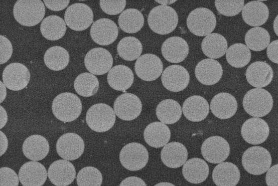
Figure-1: Polished cross section of a UD fiber composite
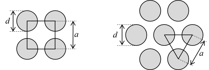
Figure-2: Square and hexagonal arrays of fibers
Square array of fibers
The fiber volume fraction of a UD composites where the fibers are arranged in a cubic array, can be derived from the cross section area fraction based on the parameters illustrated in Figure-2:
\begin{equation} V_f = \frac{A_f}{A} = \frac{ \frac{1}{4}\pi d^2 }{ a^2 } =\frac{\pi}{4}\bigg(\frac{d}{a}\bigg)^2 \tag{1} \end{equation}The maximum volume fraction is found when $d=a$ such that $V_f = \pi/4 = 0.785$
from math import pi
print(pi/4)
The configuration of the cubical array for any volume fraction can be illustrated using the function plotSquareArrayOfFibers() found in the Plot gallery:
from plotlib import plotSquareArrayOfFibers
%matplotlib inline
plotSquareArrayOfFibers(Vf=0.50)
plotSquareArrayOfFibers(Vf=0.75)


Hexagonal array of fibers
The fiber volume fraction of an hexagonal array of fibers as function of the fiber diameter and the fiber distance is
\begin{equation} V_f = \frac{A_f}{A} = \frac{\pi d^2 }{ 4 a^2\text{sin}(60)} = \frac{\pi }{ 2 \sqrt{3}}\bigg(\frac{d}{a}\bigg)^2 \tag{2} \end{equation}The maximum volume fraction is found when $d=a$ where the numerical value is
from math import pi
print(pi/(2*(3)**0.5))
Random distribution and fiber diameter variation
For a truly random distribution, a repeating unit cell (or representative volume) cannot be found. Figure 3 shows a simulated random distribution of fibers based on a sample of fibers with a given fiber diameter distribution. Details are found in the case study Fiber diameter distribution.

Figure-3: Random distribution of fibers and fiber diameter variation
Woven fabric composites
Woven fabrics are produced by the interlacing of warp (0°) fibres and weft (90°) fibres in a regular pattern or weave style. The fabric’s integrity is maintained by the mechanical interlocking of the fibers. There are several weave styles, including plain, twill, satin and basket.
Chopped strand mat (CSM)
CSM is a non-woven material consisting of randomly orientated chopped strands of glass fibers held together by chemical means. Chopped strand mat is rarely used in high performance composite components as it is impossible to produce a laminate with a high fibre content and, by definition, a high strength-to-weight ratio.
The understanding of arrangements and properties of woven fabrics and chopped strand mats is more easily acquired after the introduction of laminates and laminate theory. Relevant case studies: Eastic properties of woven plies and Eastic properties of CSM
Volume fraction versus mass fraction
Assume a composite material having two components: fibers and matrix. The total mass is
\begin{equation} m = m_f + m_m \tag{3} \end{equation}By introducing the densities of fibers and matrix, this can now be expressed by volumes:
\begin{equation} v\rho = v_f \rho_f + v_m \rho_m \tag{4} \end{equation}Since the fiber volume fraction is defined as the volume of fibers to the total volume,
\begin{equation} \rho = V_f \rho_f + V_m \rho_m \tag{5} \end{equation}Note that the $V_f + V_m = 1$ such that
\begin{equation} \rho = V_f \rho_f + (1-V_f) \rho_m \tag{6} \end{equation}The fiber volume fraction based on known mass quantities and densities of fibers and matrix is
\begin{equation} V_f= \frac{m_f \cdot \rho_m}{m_f \cdot \rho_m+m_m \cdot \rho_f} \tag{7} \end{equation}Example:
mf=50  # mass quantity of fiber
mm=50  # mass quantity of matrix

rhof = 2540 # density of a glass fiber
rhom = 1250 # density of an epoxy

Mf = (mf)/(mf+mm)
Vf = (mf*rhom)/(mf*rhom+mm*rhof)

print('The mass fraction is',Mf, 'while the volume fraction is',Vf)
Keeping the total mass equal to 100 while varying the mass of fiber:
import numpy as np
mf=np.linspace(0,100,101)
mm=100-mf
Vf = (mf*rhom)/(mf*rhom+mm*rhof)

import matplotlib.pyplot as plt
%matplotlib inline
import numpy as np

fig,ax = plt.subplots(nrows=1,ncols=1, figsize = (5,3))
ax.plot(mf,Vf,color='red',label='$V_f$')
ax.grid(True)
ax.set_xlim(0,100)
ax.set_ylim(0,1)
ax.legend(loc='best')
ax.set_xlabel('Fiber mass',size=10)
ax.set_ylabel('Volume fraction',size=10)

plt.show()

Experimental approaches
Experimental quantification of volume fractions is obviously an important issue. There are a few methods, two of them being described in this section: the burn-of method and microscopy image analysis.
Burn-off method
This method involves heating up the composite to a temperature at which the polymer matrix decomposes to a gas while the fibers, or other reinforcing elements remain. The method is useful for inorganic fibers that remain stable at elevated temperatures, such as glass, basalt and SiC-fibers. The method is generally not applicable for aramide and other polymer fibers which will decompose along with the matrix. The method is also highly questionable for carbon fiber composites due to chemical reactions that occur at elevated temperature.
The principal method and analysis is straigth forward:
- Measure the weight of the composite specimen
- Perform the matrix burn-off using a proper temperature and time for the material system
- Measure the weight of the remaining material, i.e. the fibers.
- Convert from mass to volume fraction using known values for the densities (7)
The method introduces several sources of errors, most significantly:
- A relatively moderate amount of voids has a relatively high influence on the result if not taken into acount
- The method will decompose the sizing of the fibers.
Image analysis
Optical microscopy-based techniques use representative cross-sectional images, typically recorded at several locations in the material. These images are analyzed using various algorithms. A relatively straight forward procedure is where the images are converted to a binary format as illustrated in Figure-4.
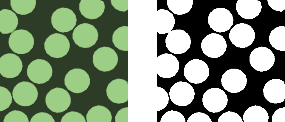
Figure-4: Converting from a microscopy image to a binary image
The following Python code demonstrates this technique:
from PIL import Image
im = Image.open("imgs/microssection.png")
im= im.convert('1') # convert image to binary image
                    # where the pixel values are either true (white) or false (black)
import numpy
a = numpy.asarray(im)  # returns the pixel values as a numpy array
imageshape=a.shape     # returns a tuple of (lines,columns)
totpix=imageshape[0]*imageshape[1]   # computing the total number of pixels
white=np.count_nonzero(a)   # this is for the fiber in the current case
print('The image shape is',imageshape,'where the total no of pix=',totpix,'and no of white pix=',white)
print('Fiber volume fraction is',white/totpix)


