Material properties
The term typical properties is frequently used about composite materials in the literature. The term is rather ambiguous when factor in all the possible variations including the different constituent materials, volume fractions, manufacturing methods, processing conditions and so forth. Some property values can be predicted fairly accurate by simple models, provided basic information about constituent materials and volume fraction. One example is the longitudinal modulus of UD fiber composites. When the volume fraction $V_f$ is known along with the modulus of the fiber $E_f$ and the matrix $E_m$, the simple rule of mixture predicts the longitudinal modulus more or less exact for any practical purposes as
$$E_1 = V_f E_f + (1-V_f) E_m$$A Python function for the model is:
def longitudinalModulus(Vf, Ef, Em):
    return Vf*Ef + (1-Vf)*Em
Now assume a composite having a E-glass fibers with a modulus $E_f$ and a matrix with modulus $E_m$, both values in the middle of the typical range, and where the fiber volume fraction is $V_f$ = 0.5:
longitudinalModulus(Vf=0.5, Ef=73, Em=3)
Commercially produced UD glass composites may have a fiber content as low as $V_f$ = 0.4. Furthermore, reported modulus for E-glass fibers is as low as 69 GPa, and common thermoset matrices with modulus of 2 GPa are available. In this case:
longitudinalModulus(Vf=0.4, Ef=69, Em=2)
Correspondingly, using upper bound values for the moduli as well as upper bound value for practical achievable fiber volume fraction give:
longitudinalModulus(Vf=0.6, Ef=76, Em=4)
Common industrial carbon fibers such as T300, T700, AS4, and AS7 have a longitudinal modulus in the range 230 – 240 GPa. The longitudinal modulus of UD composites made of these fibers where the fiber volume fraction is in the range 0.5 – 0.6 is:
E1_low= longitudinalModulus(Vf=0.5, Ef=230, Em=2)
E1_high=longitudinalModulus(Vf=0.6, Ef=240, Em=4)

print('E1, lower range: {0} GPa,   E1, upper range: {1} GPa'.format(E1_low,E1_high))
The density of composites is another parameter that is easily computed based on basic information by the relation:
$$\rho = V_f \rho_f + (1-V_f) \rho_m$$For a fiber volume fraction of 0.55 and a matrix with density equal to 1.3, the densities of E-glass, carbon and Kevlar composites are:
def compositeDensity(Vf, rhof, rhom):
    return Vf*rhof+(1-Vf)*rhom

grp=compositeDensity(0.55, 2.55, 1.35) #E-glass
crp=compositeDensity(0.55, 1.78, 1.35) #Carbon (T300,AS4, etc)
krp=compositeDensity(0.55, 1.44, 1.35) #Kevlar 29 and 49

print('E-glass:{:.2f} g/cm3, Carbon:{:.2f} g/cm3, Kevlar:{:.2f} g/cm3'.format(grp,crp,krp))
Most of the other basic material parameters of composites are more complicated to estimate. For example, the transverse moduli of UD fiber composites depends not only on the fiber volume fraction and moduli of constituent materials, but also on the 3-dimensional elastic response of the matrix, the non-isotropic nature of many of the fibers, as well as on how the fibers are distributed. Likewise, the strength parameters of composites depends on a multitude of factors, including how to interpret strength.
Nomenclature
Throughout this compendium, you will find material properties expressed in a coordinate system 1-2-3. For UD fiber composites, the 1-axis will usually correspond to the longitudinal direction of the fibers, although that is not a formal convention. The following list of parameters includes the corresponding python variables or dictionary key names for Python codes in parentheses. The parameters are described and discussed in subsequent sections of the compendium.
$V_f$ (Vf): Fiber volume fraction
$\rho$ (rho): Mass density
$E_1, E_2, E_3$ (E1, E2, E3): Young's moduli along 1, 2 and 3 directions
$v_{12},v_{13},v_{23}$ (v12, v13, v23): Poisson's ratios for 1-2, 1-3 and 2-3 interactions
$G_{12},G_{13},G_{23}$ (G12, G13, G23): Shear moduli on plane 1-2, 1-3 and 2-3
$\alpha_1,\alpha_2,\alpha_3$ (a1, a2, a3): Coefficients of thermal expansions along 1, 2 and 3 directions
$X_T, Y_T, Z_T$ (XT, YT, ZT): Tensile strengths along 1, 2 and 3 directions
$X_C, Y_C, Z_C$ (XC, YC, ZC): Compressive strengths along 1 ,2 and 3 directions
$S_{12}, S_{13}, S_{23}$ (S12, S13, S23): Shear strengths on plane 1-2, 1-3 and 2-3
Unidirectional fiber composites
Unidirectional fiber composites are assumed to be transversely isotropic, meaning that one plane is a plane of isotropy and any direction in this plane is a transverse direction (i.e. transverse to the fiber direction). The 1-axis correspond to the longitudinal direction of the fibers while the 2 and 3 axes are transverse directions. Consequently, properties in the 3-direction is equal to the properties in the 2 direction, and properties on a 1-3 plane equals properties on a 1-2 plane.
| E-glass/ Epoxy |
S-glass/ Epoxy |
Kevlar-49/ Epoxy |
Carbon/ Epoxy(a) |
Carbon/ Epoxy(b) |
|
|---|---|---|---|---|---|
| $V_f$ (-) | 0.55 | 0.55 | 0.55 | 0.55 | 0.55 |
| $\rho$ (g/cm3) | 2.0 | 2.0 | 1.4 | 1.6 | 1.7 |
| $E_1$ (GPa) | 40 | 48 | 73 | 130 | 330 |
| $E_2,E_3$ (GPa) | 10 | 11 | 5 | 10 | 8 |
| $v_{12},v_{13}$ (-) | 0.30 | 0.30 | 0.35 | 0.28 | 0.28 |
| $v_{23}$ (-) | 0.40 | 0.40 | 0.45 | 0.50 | 0.50 |
| $G_{12},G_{13}$ (GPa) | 3.8 | 4.2 | 2.2 | 4.5 | 4.0 |
| $G_{23}$ (GPa) | 3.4 | 3.6 | 1.7 | 3.5 | 2.7 |
| $\alpha_1$ (10-6/K) | 7.0 | 4.0 | -1.0 | -0.5 | -0.7 |
| $\alpha_2,\alpha_3$ (10-6/K) | 22 | 20 | 50 | 30 | 30 |
| $X_T$ (MPa) | 1000 | 1300 | 1400 | 1800 | 1000 |
| $Y_T,Z_T$ (MPa) | 40 | 40 | 20 | 40 | 40 |
| $X_C$ (MPa) | 700 | 800 | 300 | 1200 | 800 |
| $Y_C,Z_C$ (MPa) | 120 | 140 | 120 | 180 | 100 |
| $S_{12},S_{13}$ (MPa) | 70 | 70 | 40 | 70 | 70 |
| $S_{23}$ (MPa) | 40 | 40 | 20 | 40 | 40 |
Table-1: Properties of UD fiber composites
The data in Table-1 origin from partly micromechanical estimation and partly from interpolation/extrapolation and averaging of values reported in the literature. The values are partly chosen in order to indicate similarities and differences between the materials rather than to provide data for design. For that reason, the fiber volume fraction and the matrix are assumed identical for all materials.
The Carbon/Epoxy(a) has common and typical low modulus medium strength fibers such as T300, T700, AS4 and AS7, while Carbon/Epoxy(b) has high modulus (600 MPa) low strength fibers that fall in the category of graphite fibers.
As for the fibers, the specific stiffness and strength are of particular interest. The materials in Table-1 illustrated along with some high strength steel and aluminum following the procedure described in the section Fibers:
materials=[]
materials.append( {'name':'E-glass/Epoxy'         , 'rho':2.0, 'E1':  40, 'E2': 10,'XT':1000} )
materials.append( {'name':'S-glass/Epoxy'         , 'rho':2.0, 'E1':  48, 'E2': 11,'XT':1300} )
materials.append( {'name':'Kevlar-49/Epoxy'       , 'rho':1.4, 'E1':  73, 'E2':  5,'XT':1400} )
materials.append( {'name':'Carbon/Epoxy(a)'       , 'rho':1.6, 'E1': 130, 'E2': 10,'XT':1800} )
materials.append( {'name':'Carbon/Epoxy(b)'       , 'rho':1.8, 'E1': 330, 'E2':  8,'XT':1000} )
materials.append( {'name':'High strength steel'   , 'rho':7.8, 'E1': 220, 'E2':220,'XT':1500} )
materials.append( {'name':'High strength aluminum', 'rho':2.7, 'E1':  70, 'E2': 70,'XT':1000} )

names,xdata,ydata=[],[],[]
for mat in materials:
    names.append(mat['name'])
    xdata.append(mat['E1']/mat['rho'])
    ydata.append(mat['XT']/mat['rho'])

from plotlib import plotMatIndex
%matplotlib inline
plotMatIndex(names,xdata,ydata,'Specific longitudinal stiffness','Specific longitudinal strength')

Since single unidirectional layer of fiber materials rarely are used, a more realistic comparison is the one between cross-ply laminates (0/90). As a rough estimation, we can take the average of $E_1$ and $E_2$ and the half of the longitudinal tensile strength:
for i in range(0,len(names)-2): #not including steel and aluminum
    xdata[i]=xdata[i]/2
    ydata[i]=ydata[i]/2

plotMatIndex(names,xdata,ydata,'Specific cross-ply stiffness','Specific cross-ply tensile strength')

Composites are commonly found as panels and beams somehow subjected to flexural loading. The potential for very high structural efficiency, in this case, specific flexural stiffness and strength, can easilly be demonstrated by the following example:
Consider a panel, freely supported and subjected to a 3-point bending.
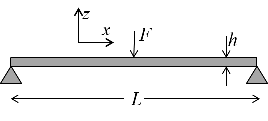
Figure-1: 3-point bending
The deflection is
\begin{equation} \delta = \frac{FL^3}{4 E b h^3} \tag{1} \end{equation}and the mass of the panel is
\begin{equation} m=Lbh\rho \tag{2} \end{equation}Assume now that the length, width, force and maximum allowable mass are all requirements that are specified. What are the deflections for the different materials?
The thickness is now a variable given by the requirements:
\begin{equation} h=\frac{m}{Lb\rho} \tag{3} \end{equation}# Requirements:
L=1 # m
b=0.1 # m
F=100 # N
m=2 # kg
# Computed thickness and deflection:
for mat in materials:
rho=mat['rho']*1E3 # kg/m3
E=mat['E1']*1E9 # Pa
h=m/(L*b*rho) # m
delta = (F*L**3)/(4*E*b*h**3)
print('{:25}: h= {:5.2f} mm, delta= {:7.4f} mm'.format(mat['name'],1000*h,1000*delta))
Hence, for a given allowable mass, the flexural stiffness of the high modulus carbon fiber composite solution is
67.4080/0.5523
times greater than the steel panel solution having the same weight.
More commonly, the maximum allowable deflection is specified. The required thickness is now
\begin{equation} h = \bigg(\frac{FL^3}{4 E b \delta}\bigg)^\frac{1}{3} \tag{4} \end{equation}and the resulting weight when using the different materials can be computed by:
# Requirement:
delta = 5E-3

# Computed thickness and mass:
for mat in materials:
    rho=mat['rho']*1E3  # kg/m3
    E=mat['E1']*1E9     # Pa
    h=((F*L**3)/(4*E*b*delta))**(1/3)     # m
    m=L*b*h*rho  # kg
    print('{:25}: h= {:5.2f} mm, m= {:7.5f} kg'.format(mat['name'],1000*h,m))
4.76/0.96
That is; the resulting mass of the steel solution is almost five times the mass of the high modulus carbon fiber composite solution.
Woven fabric composites
Woven fabrics are produced by the interlacing of warp (0°) fibres and weft (90°) fibres in a regular pattern or weave style. The fabric’s integrity is maintained by the mechanical interlocking of the fibers. There are several weave styles, including plain, twill, satin and basket.
Chopped strand mat (CSM)
CSM is a non-woven material consisting of randomly orientated chopped strands of glass fibers held together by chemical means. Chopped strand mat is rarely used in high performance composite components as it is impossible to produce a laminate with a high fibre content and, by definition, a high strength-to-weight ratio.
The understanding of arrangements and properties of woven fabrics and chopped strand mats is more easily acquired after the introduction of laminates and laminate theory. See the case studies Elastic properties of woven plies and Elastic properties of CSM
Wood
Wood may be described as an orthotropic material; that is, it has unique and independent mechanical properties in the directions of three mutually perpendicular axes: longitudinal (1), tangential (2) and radial (3). The longitudinal axis is parallel to the fiber (grain); the radial axis is normal to the growth rings (perpendicular to the grain in the radial direction); and the tangential axis is perpendicular to the grain but tangent to the growth rings.
The low density of some woods, most noteably Balsa, makes them good candidates as core materials in sandwich structures
| Balsa | Pine | |
|---|---|---|
| $\rho$ (g/cm3) | 0.16 | 0.45 |
| $E_1$ (MPa) | 3740 | 13530 |
| $E_2$ (MPa) | 56 | 1055 |
| $E_3$ (MPa) | 172 | 1529 |
| $v_{12}$ (-) | 0.49 | 0.29 |
| $v_{13}$ (-) | 0.23 | 0.33 |
| $v_{23}$ (-) | 0.23 | 0.30 |
| $G_{12}$ (MPa) | 138 | 1096 |
| $G_{13}$ (MPa) | 202 | 1109 |
| $G_{23}$ (MPa) | 19 | 176 |
Table-2:Elastic properties of wood
Python tips & tricks
Throughout this compendium, you will find materials data in Python dictionaries. Dictionaries provide a versatile, dynamic method to store structured data in an associative array. It is however easy to mess up the data due to dynamic nature of dictionaries. Therefore, some tips and tricks are warranted.
Note that the data in Table-1 are given using a mix of inconsistent units that should not be used as is in computational problems. The material E-glass/Epoxy, implemented by SI units (or Pa-m-kg) is:
grp = {'name':'E-glass/Epoxy', 'units':'Pa-m-kg', 'Vf': 0.55, 'rho':2000.0, 'E1':40.0E9, 'E2':10.0E9, 'E3':10.0E9,
       'v12':0.3,    'v13':0.3,  'v23':0.4, 'G12':3.8E9,   'G13':3.8E9, 'G23':3.4E9,
       'a1':7.0E-6, 'a2':22.0E-6, 'a3':22.0E-6, 'XT': 1000.0E6, 'YT':40.0E6, 'ZT':40.0E6,
       'XC': 700.0E6, 'YC':120.0E6, 'ZC':120.0E6, 'S12': 70.0E6, 'S13':70.0E6, 'S23':40.0E6 }
In the example above, the relevant meta-data ‘units’ is included. Additional data can be added on the fly, for example a description:
grp.update({'description':'Typical UD E-glass/Epoxy from TMM4175'})
There are many options for output listing of the data. A simple method without any explicit formatting is:
for key in grp:
    print(key,grp[key])
The next example forces the keys to occupy at least 6 characters, and '= ' is added as a pretty separation between the key and the value:
for key in grp:
    print('{:6}= {:}'.format(key,grp[key])  )
Copy using deepcopy()
One common mistake when using dictionaries (or other collections that are mutable) is to consider an assignment statement to be the creation of a copy. Assignment statements in Python do not copy objects; they create bindings between a target and an object. It may help to think of the variable assigned to a dictionary as a pointer to the dictionary object, and we may have many pointers to the same object.
For instance, assign a new parameter to the existing material, and modify the name:
grpcopy = grp

grpcopy['name']=grpcopy['name'] + ' -copy'
As expected (if you read the explanation above), the name of m1 has changed as well. After all, both m1 and m1copy point to the same object (dictionary):
print(grp['name'])
print(grpcopy['name'])
The simple solution is to use deepcopy():
grp['name']='E-glass/Epoxy'

from copy import deepcopy

grpcopy=deepcopy(grp)
grpcopy['name']=grpcopy['name']+'-copy'
Now the two variables point to two different dictionaries:
print(grp['name'])
print(grpcopy['name'])
Unit conversion
Although the consistent SI system of units is simple and safe to use, the MPa-mm-Mg system (also consistent) is often more convenient for engineering problems, simply due to the more readable size of the numbers. Sophisticated algorithms for converting between different systems can be made. The example below applies only for the particular conversion from Pa-m-kg to MPa-mm-kg, and a new material is returned by the function:
def unitConvert_Pa_MPa(m):
    from copy import deepcopy
    mcopy=deepcopy(m)
    # the possible items having unit Pa:
    convMPa = ('E1','E2','E3','G12','G13','G23',
               'XT','YT','ZT','XC','YC','ZC','S12','S13','S23')
    if m['units']=='MPa-mm-Mg':
        return mcopy  # nothing to convert here
    if m['units']=='Pa-m-kg':
        for key in mcopy:
            if key in convMPa:
                mcopy[key]=mcopy[key]*1E-6
            if key=='rho':
                mcopy['rho']=mcopy['rho']*1E-12
            mcopy['units']='MPa-mm-Mg'
        return mcopy
    else:
        return 'Do not know what to do' # messed up units label or something..
Try:
grpMPa=unitConvert_Pa_MPa(grp)

for key in grpMPa:
    print('{:6}:{:}'.format(key,grpMPa[key])  )
Verify data
Computational problems require certain data, and they must be consistent. For example, 3D stress-strain problems must have a complete set of elastic constants. Furthermore, for physical consistency, there are several requirements on the elastic constants, one of them being that they must all be positive. The following example provides a verification of these requirements:
def verifyElastic3D(m):
    elastic3D = ('E1','E2','E3','G12','G13','G23','v12','v13','v23')
    moduli3D  = ('E1','E2','E3','G12','G13','G23')
    for e in elastic3D:
        if e not in m:
            return False # one or more is missing
    for e in moduli3D:
        if m[e]<=0:
            return False # moduli must be greater than zero
    return True # otherwise, it's OK
print(verifyElastic3D(grpMPa))
A simpler way to define a material
Dictionaries are a bit cumbersome to write. The following function provides a more convenient way involving less typing:
def newMaterial(**kwargs):
    m={}
    for key in kwargs:
        m.update({key:kwargs[key]})
    return m
The **kwargs in the function definitions in python is used to pass a keyworded, variable-length argument list, and the function returns a material as a dictionary.
m1=newMaterial(name='Cryptonite', E1=40, E2=10, E3=10, v12=0.3, v13=0.3, v23=0.5, G12=3, G13=3, G23=3)

print(m1)
Material library
A solution for a material library is suggested in Material Library. Many examples in this compendium will load materials from the library and it is probably worthwhile to figure out how to utilize this way of organizing materials for your own work and studies.


