Finite element analysis
The finite element method (FEM) is a powerful technique for numerical solution of complex problems in structural mechanics, and it remains the method of choice for complex systems. In the FEM, the structural system is modeled by a set of appropriate finite elements interconnected at discrete points called nodes. Elements have physical and geometrical properties which may include density, thickness or cross section, as well as mechanical propertes such as elastic properties.
Finite element analysis (FEA) as applied in engineering is a computational tool for performing engineering analysis. It includes the use of mesh generation techniques for dividing a complex problem into small elements, as well as FEM algorithms (solvers) and postprocessing tools for the results.
Some of the well known commercial software packages include Abaqus, Ansys, Comsol, LS-DYNA and Nastran, among others.
In TMM4175 Lighteweight Design, we will be using Abaqus. Detailed information about availability, download and installation can be found in the course information.
Additional information and examples, see Abaqus Scripting
Guidelines to a systematic approach
The options, methods and level of details for finite element models and analyses of mechanical problems are close to infinite. Hence, reasonable choices must be made at every steps in the process. The scale in question, the level of resolution, the level of accuracy, are all determined by the choices made and the options employed. There will always be a trade-off between the demand for precision and the modelling and analysis cost (e.g. computational time). Application of FEA can probably be considered as both art and science, where the art part requires a lot of experience and acquired skills.
This brief introduction to a systematic approach is partly generic, however not comprehensive. The objectives are to provide an essential guide for the course TMM4175. Hence, lightweight design and composite modelling and analyses are emphasized whenever relevant.
Most of the examples in the course make use of the N-mm-s-Mg system. The reason behind this choice is purely based on convenience. When using the N-mm-s-Mg system, you must pay attention to all the input variables and properties in a systematic way.
| N-m-s-kg | N-mm-s-Mg | Factor | |
|---|---|---|---|
| Length | m | mm | 103 |
| Force | N | N | 100 |
| Time | s | s | 100 |
| Mass | kg | Mg | 10-3 |
| Volume | m3 | mm3 | 109 |
| Density | kg/m3 | Mg/mm3 | 10-12 |
| Stress | Pa | MPa | 10-6 |
| Pressure | Pa | MPa | 10-6 |
| Modulus | Pa | MPa | 10-6 |
| Moment | Nm | Nmm | 103 |
| Acceleration | m/s2 | mm/s2 | 103 |
| Gravity | m/s2 | mm/s2 | 103 |
| Energy | J | mJ | 103 |
The scale of the problem
The scope with respect to the scale, or the resolution of the results, should be carefully assessed for each specific case question.
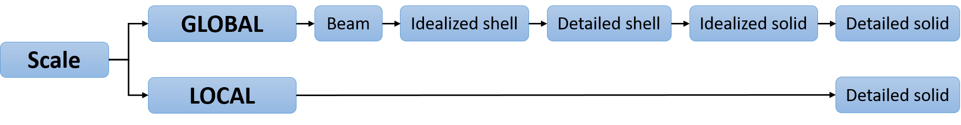
Global response
For example, the tip deflection of a cantilever beam can potentially be obtained very accurately (and extremely efficiently) using a beam element model. If not, an idealized shell model, or a more detailed shell model must be considered. If the beam contains local details that really govern the global response, a solid model with a sufficient degree of details should be considered.
Local effects and results
A detailed solid model is typically required where three dimensional state of stress exists, and this stress state is of relevance for the problem, typically for detailed strength and material failure assessment.
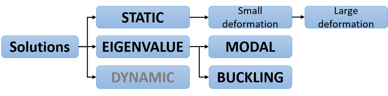
Solutions
The relevant types of analysis (Abaqus: Step) for the problem must be identified, and these are obviously deduced from the defined function and requirements of the structure. Static analyses are typically used to solve real static load cases, but can often be successfully employed to solve dynamic problems as well, for example by introducing dynamic factors for loads when the dynamics of the structure is relatively simple and well understood. Eigenvalue solutions represents cost efficient methods for assessing buckling and vibrations in a linearized way.
Composite structures
Composite structures are often found as components and assemblies having thin shells and slender structural members. They are often used when large deformation is an intrinsic feature (such as a wing, a bow or spring-like structures) and they are often prone to buckling where compressive loads are present in a section. Modal, frequency analyses may serves several purposes, but the most common one is to design the structure in a way that avoid resonance with identified cyclic loading. Dynamic solutions (implicit/explicit) are not discussed further in the course, although being very relevant for the real life.
Relations to the scale in question:
Typically, but not exclusively, the eigenvalue problems are relevant on the global scale where the model needs to be sufficiently accurate with respect to stiffness, and be able to capture the most critical modes.
Element types
The different elements come with pros and cons, and the choice will be a result of many trade-offs. Generally, your initial choices should be the default (and recommended) types. Then, based on issues discovered during the work, you may arrive to different choices.
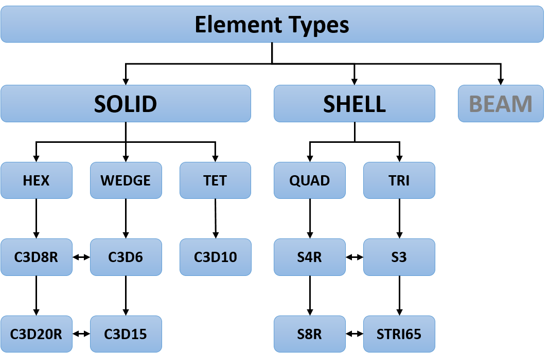
Solids
Whenever possible, use linear HEX with reduced integration (Abaqus: C3D8R). This element can be combined with WEDGE elements (Abaqus: C3D6). If TET elements are the only option, use quadratic elements (Abaqus: C3D10). For linear HEX with reduced integration you must pay attention to hour-glassing as well as poor representation of bending stiffness for sections having few elements through the thickness.
Shells
The linear QUAD with reduced integration (Abaqus: S4R) is the default choice and suitable for most problems. The element can be combined with S3, but the number of TRI elements should be minimized, and preferably avoided altogether.
Beams
Beam elements are somewhat relevant but not included in the course.
Composites and laminates
TET elements have minor relevance in composite modelling, and are particularly inapplicable for modelling layered structures, both in discrete manner and by layered element definition (Abaqus: Composite Layup)
Layered structures
The most useful approach for the representation of a layered structure is obviously very dependent on the scale in question. Models and analyses with a global scope will usually take a layered shell or layered solid approach as the initial, default option. The discrete approach is generally limited to cases where complex stress states and high stress and strain gradients are present at the laminate and layer scale. Examples includes laminate edges and detailed features such as joints and interactions with other components.
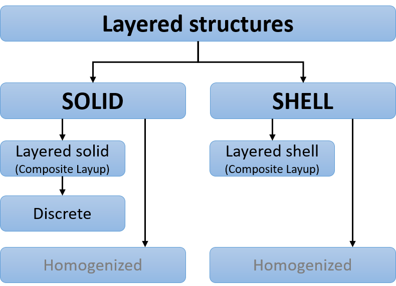
Advanced homogenized approaches are not included in the course. Note however, that the layered solid/layered shell approaches are fundamentally based on homogenization methods at the element scale.
Loads and boundary conditions
Some of the most relevant loads and boundary conditions are included in the illustration. Although these are usually straight forward and easy to interpret for mechanical engineers, there are some critical issues that needs to be addressed:
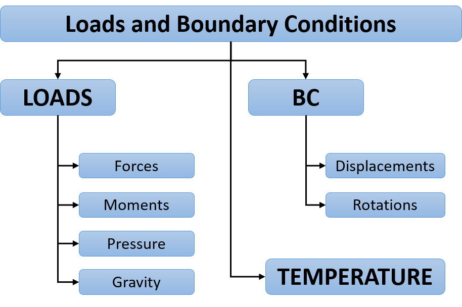
- Realistic implementation of loads and boundary conditions involves a careful assessment of the problem, and there will often be a significant uncertainty. In such cases you should study the effect by considering for example lower bound and upper bound solutions for the constrains.
- Note that the nodes of solid elements do not have rotational degree of freedom coupled to the element behavior. Both input and output for rotation of nodes are given by radians.
- Distributed loading such as pressure and body forces such as gravity is directly related to mass and geometrical features. Make sure that the combinations of parameters and options are consistent.
- Assumptions based on symmetry, periodicity and similar should be evaluated carefully. For composite materials this is often a source of error: For a symmetric condition to be true, both the geometry, the loading and the material and orientation must satisfy the symmetry condition.
- Temperature (difference) is considered as a load in mechanical analysis by its relation to thermal strains.
Results
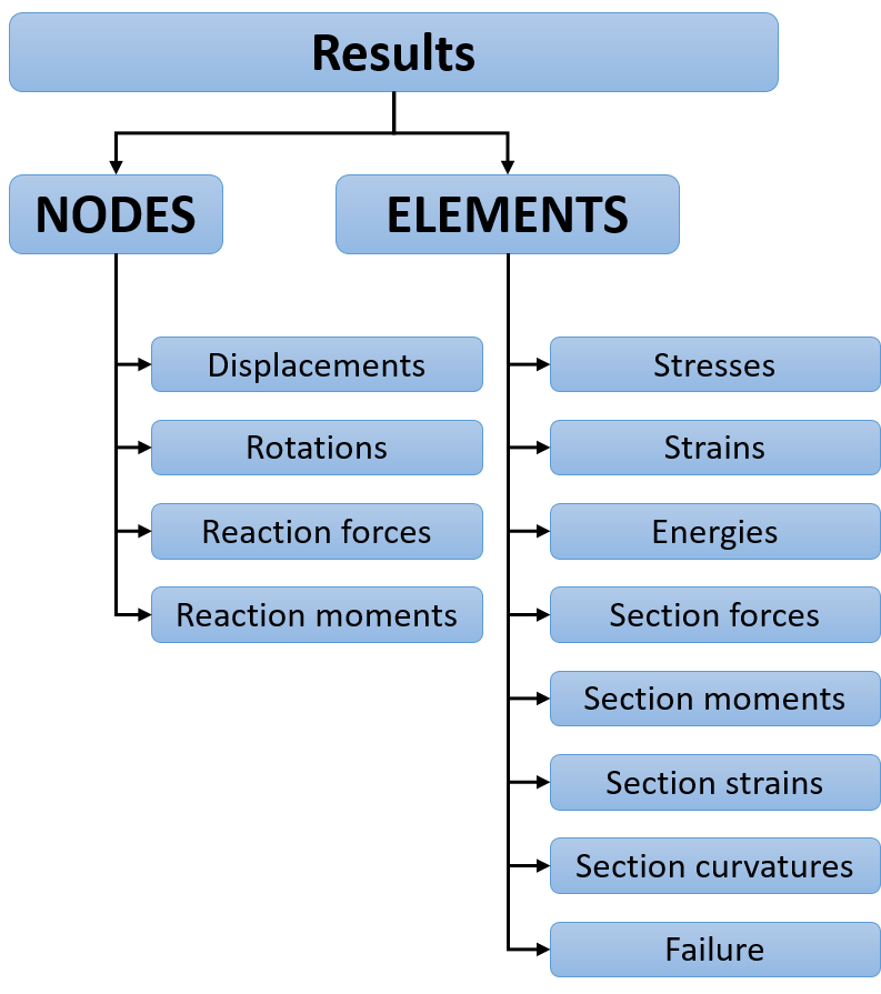
Nodal results
The basic nodal results includes displacement, rotation, forces and moments. Note that solid elements do not have rotational degree of freedom, and will not have results for reaction moments.
Elemental results
Results associated by the elements are primarily those computed at integration points, such as stresses, strains and all the derived quantities from those. Since the results are only computed at the integration point, a linear HEX with reduced integration has only one position where results are directly available. Typically, representation of results (such as contour plot) uses various forms of interpolation and extrapolation of results. The validity of such interpolation or extrapolation should be evaluated carefully. In most systems, the results are given in the material coordinate system for anything but isotropic materials.
Composite structures
Section results (forces, moments, strains and curvatures) are particularly relevant due to the direct connection to the laminate theory. For layered elements, results can be computed at several locations through the thickness of individual layers. Various failure indices (exposure factors) based on different failure criteria are available as well. These must typically be explicitly specified (Abaqus: Field Output Request)