Safety and uncertainty
It is, basically, all about probability of failure and acceptable risk in terms of life, health, money, reputation and so on.
We may come quite far with just a bit of common sense in engineering. However, the average human brain is not that intuitively precise when it comes to ridiculously large, or small, numbers involved in statistical assessment. Fortunately, the theories of statistics and probability are well developed and relatively accessible for engineers, and even better, all the failure and safety stuff have been massaged and put into simple relations, factors and tables found in guidelines and standards.
For a starter, let’s discuss the Penguin pedestrian bridge in Sharkland Zoo.
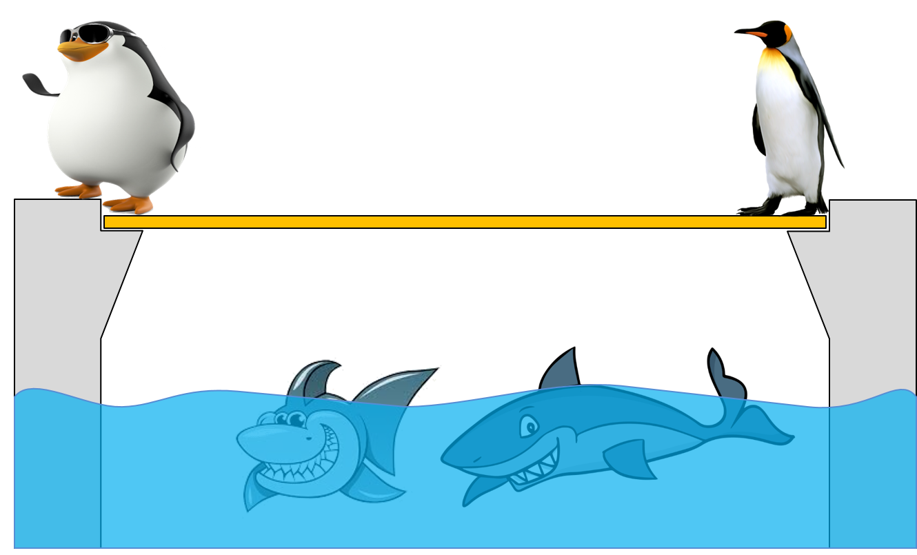
Figure-1: Penguin pedestrian bridge
The average weight of penguins at Sharkland is 15 kg, and it has been found that masses across the whole population of adults allowed crossing the bridge follows a normal probability distribution where the COV is 10% and therefore, the standard deviation is 1.5 kg.
Let us assume that only one penguin can cross at a time such that the system can be approximated to a freely supported beam in a 3-point bending configuration. These slow moving creatures do not induce any dynamics on the system so the mass of one penguin is therefore the load acting on the bridge, and worst case scenario is when the penguin is half way across the bridge. Furthermore, assume that the scatter of the load is equal to the distribution of mass illustrated in Figure-2.
Something fishy here (beyond the obvious for the location)? In order for the last assumption to be true, we must claim that Fat Pengo is just as likely to cross the bridge as Skinny Pengana. If not so, the distribution of load does not correspond to the distribution of mass since bias is being introduced into something initially assumed to be random and following a normal distribution.
You may intuitively think that Pengo is lazy and therefore less likely to cross the bridge. Well, that is another layer of bias, shame on you, which may turn out to be faulty. Maybe Pengo is fat because crossing the bridge is rewarded with more fish.
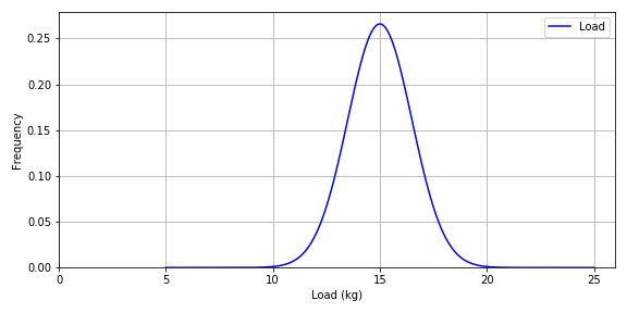
Figure-2: Mass distribution for Penguin population
The bridge shall be made of some brittle recycled plastics. The material has been extensively tested to obtain a mean strength of 40 MPa and a COV equal to 8% such that the standard deviation is 3.2 MPa as illustrated in Figure-3.

Figure-3: Strength distribution
The span length of the beam is $L=2000$ mm, the widht is $b = 100$ mm and the thickness $h$ is to be decided. The maximum tensile stress located at the mid-span in the beam is
\begin{equation} \sigma_{max} = \frac{3FL}{2bh^2} \tag{1} \end{equation}The required thickness $h$ is therefore
\begin{equation} h = \Big(\frac{3FL}{2b\sigma}\Big)^{1/2} \tag{2} \end{equation}where $\sigma$ is the allowable stress.
In the following example, the load is taken to be equal to the mean penguin mass while the allowable stress is equal to the mean strength:
m  =  15        # Mass of Penguins, mean value (kg)
L  =  2000      # Support span (mm)
b  =  100       # Width (mm)
sm =  40.0      # Mean strength (MPa)
F  =  m*9.8     # Force (N)
sa =  sm        # Allowable stress equal to mean strength (MPa)

h = ((3*F*L)/(2*b*sa))**(1/2)
print('Required thickness =',h,'mm')
It is very useful to use resistance, in terms of the mass the bridge can resist, rather than material strength for the subsequent discussion: The mean resistance for the specific design given above, is 15 kg and COV = 8% given for the material strength applies for the resitance as well. Now we can compare the two distributions directly:
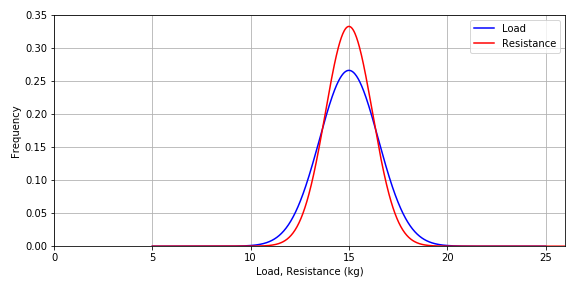
Figure-4: Load and resistance distributions
So, what is the probability of failure for this design? Intuitively, we can easily figure out that it is just as likely that the resistance is less than the strength than vices versa, and therefore, the probability of failure is $P(f)=0.5$ (by common sense!)
When both the resistance and the load follow a normal distribution, the probability of failure can easily be calculated by the standard normal cumulative distribution function $\Phi$ as
\begin{equation} P(f)=\Phi(\beta) \tag{3} \end{equation}where
\begin{equation} \beta = \frac{ \mu_L - \mu_R}{ \sqrt{\sigma_L^2 + \sigma_R^2} } \tag{4} \end{equation}and $\mu_L, \mu_R$ are mean values of load and resistance respectively, and $\sigma_L, \sigma_R$ are standard deviations (not to be confused with stresses).
from scipy.stats import norm

covL, covR   =  0.1,  0.08                  # COV values (not %!)
meanL, meanR = 15.0, 15.0                   # mean values
stdL, stdR =   meanL*covL, meanR*covR       # standard deviations

B = ( meanL - meanR )/( (stdL**2 + stdR**2)**(1/2) )

pf = norm.cdf( B )                          # norm.cdf(x) is the normal cumulative distribution function where default
                                            # value for mean is zero and standard deviation is one.

print('Probability of failure = ',pf)
A probability of failure equal to 0.5 is hard to defend, both economically (penguins are not cost efficient shark food), emotionally (penguins are cute creatures) and from concerns for the zoo’s reputation (penguins are still very cute).
How will a resistance/load-factor of 1.2 save penguin lives and urban people’s emotions?
m  =  15        # Mass of Penguins, mean value (kg)
L  =  2000      # Support span (mm)
b  =  100       # Width (mm)
sm =  40.0      # Mean strength (MPa)
F  =  m*9.8     # Force (N)
sa =  sm/1.2    # Allowable stress equal to mean strength divided by the resitance/load factor

h = ((3*F*L)/(2*b*sa))**(1/2)
print('Required thickness =',h,'mm')
The mean resistance in terms of mass (kg) is now
print(m*1.2)
For this new design, the probability of survival is obviously greater than the probability of failure:
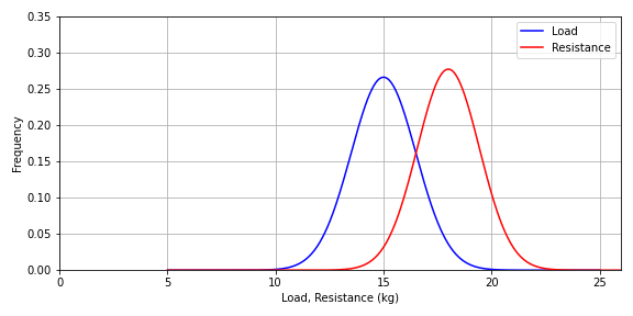
Figure-5: Load and resistance distributions
However, as apparent from the overlapping distributions, the probability of failure is still very high for everything but cheap toys and gadget deliberately designed for a short life where safety concerns are not a part of the equation at all.
What should be the resistance of the bridge if the probability of failure should be equal to 1E-6 (one out of a million)? With some iteration we arrive to this result:
covL, covR   =  0.1,  0.08                  # COV values (not %!)
meanL, meanR = 15.0, 27.71                  # mean values
stdL, stdR =   meanL*covL, meanR*covR       # standard deviations

B = ( meanL - meanR )/( (stdL**2 + stdR**2)**(1/2) )
pf = norm.cdf( B )
print('Probability of failure = ',pf)
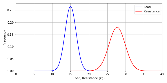
Figure-5: Load and resistance distributions
The design thickness for this probability of failure is now
m  =  27.71     # Required resistance (kg)
L  =  2000      # Support span (mm)
b  =  100       # Width (mm)
sm =  40.0      # Mean strength (MPa)
F  =  m*9.8     # Force (N)

h = ((3*F*L)/(2*b*sm))**(1/2)
print('Required thickness =',h,'mm')
print('Resistance/Load-factor =', 27.71/15.0, 'based on mean values.')
The factor 1.84 is now effectively a combined load and resistance safety factor for a probability of failure equal to 1E-6 where mean values for load and strength apply as design load and design strength. Generally, a safety factor is based on this kind of calibration targeting a defined probability of failure (corrolated to a safety level) as well as estimations of all uncertainties related to the data, assumptions, computational methods and other approximations and/or simplifications.
NOTE: This example includes a number of assumptions, like absolute confidence in the data (distributions), which hardly ever is the case for real life engineering problems. This is further discussed in the next section on Material variability and characteristic strength
Left as exercise: Suppose that we know, with absolute certainty, that the maximum load is equal to 20 kg (that is the heaviest penguin at the zoo and it is 100% probable that this penguin will cross the bridge at some time). What is the probability of failure for a bridge designed with a thickness equal to the last design (14.27 mm)?
Material variability and characteristic strength
Material variability refers to the natural or induced differences in the properties and behavior of materials. These variations can arise from factors such as raw material inconsistencies, processing methods, environmental conditions, or manufacturing tolerances.
The extent of material variability differs significantly across various materials and material groups. For example, aggregate ceramics such as stoneware and concrete, as well as natural materials like wood, exhibit a high degree of scatter in properties such as tensile strength. In contrast, standardized engineering steels show minimal variation in yield strength, reflecting their highly controlled production processes and consistent material properties.
Characteristic strength
In most design codes, material or component strength values are based on the concept of a characteristic value. The characteristic value is defined as the value below which not more than a specified percentage of the test results may be expected to fall based on the assumed distribution function. Normal distribution is most commonly employed for characteristic strength and will be used here. Note however that the basic principles applies to other distribution functions as well.
Example: Assume that the following data sample is the experimental results of a strength parameter:
v = [543.8, 507.2, 521.9, 485.8, 481.7, 528.7, 506.6, 499.1, 493.2, 392.4, 540.9, 492.1, 511.1, 457.1, 535.1, 506.0,
     573.2, 454.5, 534.6, 519.9, 570.4, 520.2, 482.7, 580.9, 573.8, 478.0, 572.6, 552.0, 534.6, 563.4, 455.2, 480.3,
     543.8, 572.3, 496.0, 495.3, 502.5, 537.7, 426.4, 456.4, 516.7, 526.5, 532.0, 536.0, 377.1, 508.4, 581.1, 540.5,
     532.5, 430.9, 483.3, 385.1, 491.7, 511.8, 465.0, 495.6, 553.1, 562.9, 545.0, 485.9, 544.5, 416.7, 538.5, 413.3,
     540.3, 541.1, 577.5, 588.1, 560.3, 505.4, 537.0, 546.7, 556.9, 513.5, 565.6, 518.7, 462.1, 548.8, 502.7, 530.8,
     500.3, 517.9, 508.1, 560.4, 569.4, 484.3, 489.6, 540.9, 540.1, 578.3, 475.7, 416.9, 519.8, 477.4, 483.0, 603.8,
     521.9, 496.1, 526.5, 516.9, 551.1, 494.2, 439.9, 584.0, 458.7, 463.7, 464.8, 520.5, 489.1, 513.0, 520.1, 509.5,
     540.9, 579.8, 478.5, 604.8, 503.9, 565.2, 462.6, 485.0, 589.4, 507.3, 560.6, 453.5, 456.5, 513.5, 416.4, 543.9,
     446. , 509.5, 544.4, 509.5, 499.8, 506.4, 585.7, 579.9, 544.0, 531.9, 529.8, 629.4, 574.8, 570.2, 512.2, 574.7,
     541.6, 483.9, 520.1, 480.7, 605. , 571.5, 587.9, 613.6, 510.2, 615.6, 517.6, 631.1, 518.4, 630.6, 492.7, 523.3,
     583.6, 474.7, 419.5, 570.8, 582.6, 463.6, 506.3, 496.7, 520.3, 559.8, 519.4, 551.6, 515.7, 598.9, 423.1, 543.2,
     555.7, 586.9, 539.9, 481.7, 479.5, 451.2, 554.3, 491.9, 522.3, 542.5, 442.5, 537.5, 604.0, 447.0, 498.4, 627.4,
     595.8, 526.2, 543.3, 573.5, 551.5, 558.3, 450.3, 567.7]
Some basic statistical parameters:
import numpy as np
import matplotlib.pyplot as plt
%matplotlib inline
from scipy.stats import norm

n    =  len(v)
vmin =  np.amin(v)
vmax =  np.amax(v)
vmean=  np.mean(v)
vstd =  np.std(v,ddof=1)
vcov =  100*vstd/vmean

print('Sample size:',n)
print('Min:        ',vmin)
print('Max:        ',vmax)
print('Mean:       ',vmean)
print('Stdev:      ',vstd)
print('COV%:       ',vcov)
Thus, the mean value is about 521 while the standard deviation is close to 50 and the coefficient of variation is 9.6 %.
We may plot the normal distribution of these data based on the mean and the standard deviation along with a histogram using 10 bins of the data:
x=np.linspace(vmin-3*vstd,vmax+3*vstd,1000)
y=norm.pdf(x,vmean,vstd)
fig,ax = plt.subplots(figsize=(10,4))
ax.plot(x,y,color='black')
n,bins,patches=plt.hist(v, bins=10, density=True,facecolor='orange', alpha=0.6 )
ax.set_xlabel('Strength')
ax.set_ylabel('Frequency')
ax.set_title('Normal distribution of strength')
ax.set_xlim(0,)
ax.set_ylim(0,)
ax.grid(True)
plt.show()

Many standards takes, for historical reasons, the 5th percentile as the characteristic strength. That is: no more than 5% of the values shall fall below this value. For a normal distribution the value is found by
\begin{equation} strength = mean - z \cdot std \tag{5} \end{equation}where $z = 1.645$
Other standards may use for example the 2.5th percentile where $z = 1.960$.
Both examples are computed and illustrated below:
p050 = vmean-1.645*vstd
p025 = vmean-1.960*vstd

fig,ax = plt.subplots(figsize=(10,4))
ax.plot(x,y,color='black')
ax.plot((p050,p050),(0,max(y)),'--', color = 'blue',label='5th percentile')
ax.plot((p025,p025),(0,max(y)),'--', color = 'red',label='2.5th percentile')
ax.set_xlabel('Strength')
ax.set_ylabel('Frequency')
ax.set_title('Normal distribution of strength')
ax.set_xlim(0,)
ax.set_ylim(0,)
ax.grid(True)
ax.legend(loc='best')
plt.show()

print('5th percentile:  ',p050)
print('2.5th percentile:',p025)

So far, the assumption of an infinite sample size (infinite number of tests) has been made. That is obviously not a viable requirement, and the statistical approach must somehow include considerations for limited sample sizes based on required confidence.
The following table is an example for the 2.5th percentile with 95% confidence:
| Sample size $n$ | $z$ |
|---|---|
| 3 | 9.0 |
| 4 | 6.0 |
| 5 | 4.9 |
| 6 | 4.3 |
| 10 | 3.4 |
| 15 | 3.0 |
| 20 | 2.8 |
| 25 | 2.7 |
| $\infty$ | 2.0 |
Table-1: Value of z for 2.5th percentile with 95% confidence
Let’s choose a 'random' sequence of 5 tests extracted from the data set:
v1 = v[15:20]
print(v1)
v1min  =  np.min(v1)
v1max  =  np.max(v1)
v1mean =  np.mean(v1)
v1std  =  np.std(v1,ddof=1)
v1cov  =  100*v1std/v1mean
v1char =  v1mean-4.9*v1std

x1=np.linspace(v1min-3*v1std,v1max+3*v1std,1000)
y1=norm.pdf(x,v1mean,v1std)
fig,ax = plt.subplots(figsize=(10,4))
ax.plot(x1,y1,color='black')
ax.plot((v1char,v1char),(0,max(y1)),'--', color = 'red',label='Characteristic strength')
ax.set_xlabel('Strength')
ax.set_ylabel('Frequency')
ax.set_title('Normal distribution of strength')
ax.set_xlim(0,)
ax.set_ylim(0,)
ax.grid(True)
ax.legend(loc='best')
plt.show()

print('Mean:                 ',v1mean)
print('Stdev:                ',v1std)
print('COV%:                 ',v1cov)
print('Characteristic value: ',v1char)

Hence, the estimated characteristic strength for the limited data set is much less than the estimation from the big data set (305 versus 423) when reasonably approximated that a sample size of 200 is close to infinite in this context.
The following code picks 195 different samples, each with a sample size of 5. The characteristic value is computed for each and shown in the graph:
cvs = []
for i in range (0,195):
    vt = v[i:i+5]
    cv = np.mean(vt) - 4.9*np.std(vt,ddof=1)
    cvs.append(cv)

fig,ax = plt.subplots(figsize=(10,4))
ax.plot(cvs,color='black')
ax.set_xlabel('Sample number')
ax.set_ylabel('Characteristic value')
ax.grid(True)
plt.show()

The result shows different estimations of characteristic strength, from approximately 130 to a maximum of about 460 depending on the chosen sub-sample. Notice however that the maximum value of 460 is relatively close to the characteristic value from the whole dataset (423). After all, the confidence is not 100% and the z- value should probably be slightly more than 2 for the large sample set. Therefore, it is perfectly reasonable that there exists sample sizes of 5 with slightly higher characteristic values than the one estimated from the whole set.
Example of bad luck picking a sequence of five specimen from the 200 specimen sample:
v2 = v[44:49]

v2min  =  np.min(v2)
v2max  =  np.max(v2)
v2mean =  np.mean(v2)
v2std  =  np.std(v2,ddof=1)
v2cov  =  100*v2std/v2mean
v2char =  v2mean-4.9*v2std

x2=np.linspace(v2min-3*v2std,v2max+3*v2std,1000)
y2=norm.pdf(x2,v2mean,v2std)
fig,ax = plt.subplots(figsize=(10,4))
ax.plot(x2,y2,color='black')
ax.plot((v2char,v2char),(0,max(y2)),'--', color = 'red',label='Characteristic strength')
ax.set_xlabel('Strength')
ax.set_ylabel('Frequency')
ax.set_title('Normal distribution of strength')
ax.set_xlim(0,)
ax.set_ylim(0,)
ax.grid(True)
ax.legend(loc='best')
plt.show()

print('Mean:                 ',v2mean)
print('Stdev:                ',v2std)
print('COV%:                 ',v2cov)
print('Characteristic value: ',v2char)

Large scatter
Materials with extensive heterogeneity on the macro scale and intrinsically brittle materials like many of the ceramics may show a large, or even a very large coefficient of variation (COV). Even the scatter of the average values of a number of series of measurements may show a large scatter compared to the overall average value. In those cases, expression (1) can easily lead to a nonsensical characteristic or minimum strength as demonstrated in the following example:
v3 = [200.0, 250.0, 300.0, 350.0, 400.0]

v3mean=  np.mean(v3)
v3std =  np.std(v3,ddof=1)
v3cov =  100*v3std/v3mean
print('Mean:                 ',v3mean)
print('Stdev:                ',v3std)
print('COV%:                 ',v3cov)
print('Characteristic value: ',v3mean-4.9*v3std)     # z = 4.9 when n = 5
Note: For most structural engineering materials including engineering metals and composites, the coefficient of variation (COV) for samples of well prepared specimen is less than 15% and the principles behind equation (1) are applicable.
Strength measurements series where large scatter is an intrinsic feature of a material or a structure may be described by 2-parameters Weibull distributions that indicate that the minimum value approaches to zero. The strength is now defined, or chosen, based on an accepted probability of failure.


