Stress
The components of stress at a point are the forces per unit area acting on planes passing through the points. The tensor notation, or Einstein notation for stress is $\sigma_{ij}$ where $i,j=1,3,4$. The first index corresponds to the direction of the normal to the plane of interest and the second index corresponds to the direction of the force as illustrated in Figure-1 (left).
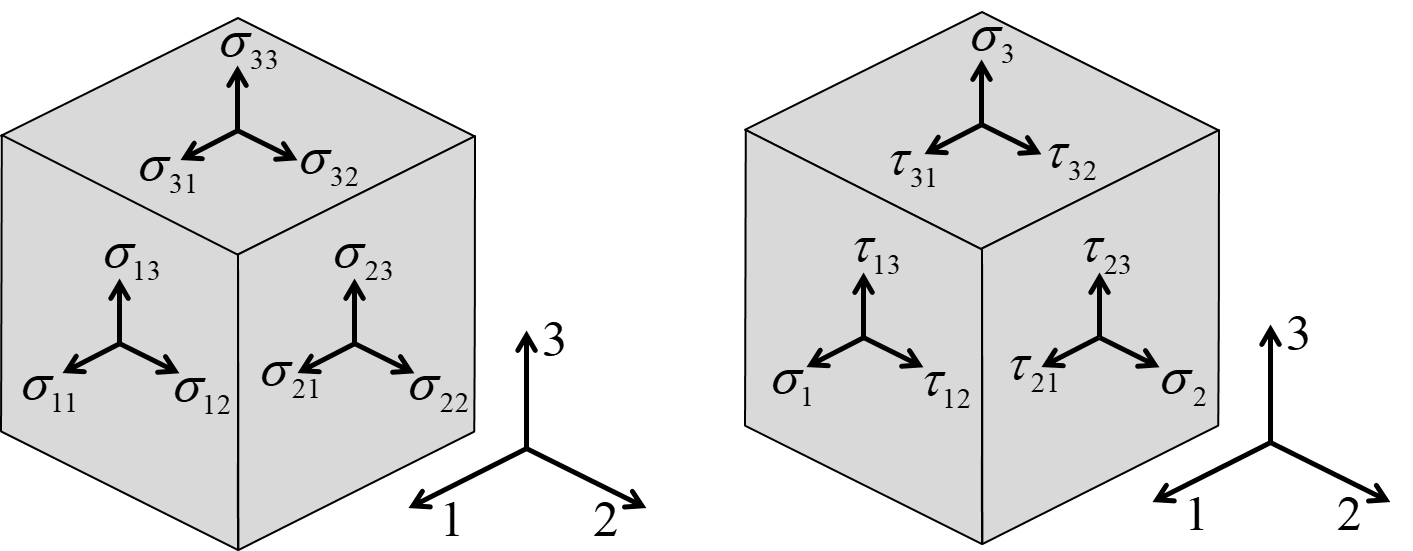
Figure-1: Components of stress in a 1,2,3 koordinate system
The stress tensor can be written as a 3 x 3 matrix:
\begin{equation} \boldsymbol{\sigma}= \begin{bmatrix} \sigma_{11} & \sigma_{21} & \sigma_{31} \\ \sigma_{12} & \sigma_{22} & \sigma_{32} \\ \sigma_{13} & \sigma_{23} & \sigma_{33} \end{bmatrix} \label{eq:stresstensor1} \tag{1} \end{equation}Force and moment equilibrium requires that the stress tensor to be symmetric (i.e., $\sigma_{ij}=\sigma_{ji}$). Furthmore, we will follow the common practice to use the notation $\tau_{ij}$ for shear stresses and use reduced notation for normal stresses (i.e., $\sigma_{ii}=\sigma_i$). Hence, the stresses by the simplified matrix notation becomes
\begin{equation} \boldsymbol{\sigma}= \begin{bmatrix} \sigma_{1} & \tau_{12} & \tau_{13} \\ \tau_{12} & \sigma_{2} & \tau_{23} \\ \tau_{13} & \tau_{23} & \sigma_{3} \end{bmatrix} \label{eq:stresstensor2} \tag{2} \end{equation}Due to the symmetry, there are only 6 independent components of stress.
In a coordinate system x,y,z as illustrated in Figure-2, the stress is written
\begin{equation} \boldsymbol{\sigma}= \begin{bmatrix} \sigma_{x} & \tau_{xy} & \tau_{xz} \\ \tau_{xy} & \sigma_{y} & \tau_{yz} \\ \tau_{xz} & \tau_{yz} & \sigma_{z} \end{bmatrix} \label{eq:stresstensor3} \tag{3} \end{equation}
Figure-2: Components of stress in a x,y,z coordinate system
If the concept of stress somehow gone under the radar during your materials and mechanical engineering studies, an introductory textbook on mechanics of materials, for example [1] will provide the proper background
Consider a stress state
$$ \boldsymbol{\sigma}= \begin{bmatrix} \sigma_{x} & \tau_{xy} & \tau_{xz} \\ \tau_{xy} & \sigma_{y} & \tau_{yz} \\ \tau_{xz} & \tau_{yz} & \sigma_{z} \end{bmatrix}= \begin{bmatrix} 100 & 20 & 0 \\ 20 & 50 & 0 \\ 0 & 0 & 0 \end{bmatrix} $$A straight forward NumPy-array representation is:
import numpy as np

sigA=np.array ( [ [  100.0,  20.0,   0.0   ],
                  [     20.0,  50.0,   0.0 ],
                  [      0.0,   0.0,   0.0 ] ])

print(sigA)
The stress state above is an example of a plane stress case (stress exsists only on the 1-2 plane), while the two examples that follow are pure shear ($\tau_{yz} \ne 0$) and pure pressure ($\sigma_x=\sigma_y=\sigma_z=-P$) respectively:
sigB=np.array ( [ [ 0.0,   0.0,   0.0 ],
                  [ 0.0,   0.0,  50.0 ],
                  [ 0.0,  50.0,   0.0 ] ] )

sigC=np.array ( [ [-20.0,   0.0,  0.0 ],
                  [  0.0, -20.0,   0.0 ],
                  [  0.0,   0.0, -20.0 ] ] )

print(sigB)
print()
print(sigC)
Eigenvalues and eigenvectors
The eigenvalues $\lambda$ and the eigenvectors $\mathbf{v}$ are the solutions of \begin{equation} (\boldsymbol{\sigma}-\mathbf{I}\lambda)\mathbf{v}=\mathbf{0} \label{eq:eigenv} \tag{4} \end{equation}
Plane stress example where $\sigma_z=\tau_{xz}=\tau_{yz}=0$ :
sig=np.array ( [ [ 100.0,  20.0,  0.0 ],
                 [  20.0,  50.0,  0.0 ],
                 [   0.0,   0.0,  0.0 ] ] )

L,v = np.linalg.eig(sig)

print('Eigenvalues:')
print(L)
print()
print('Eigenvectors:')
print(v)
Note that the eigenvectors are the given by columns and thus it is more convenient to do a transpose:
v = v.T
for vi in v:
    print(np.round(vi,3))
Verify that equation (4) is true by computing \begin{equation} (\boldsymbol{\sigma}-\mathbf{I}\lambda)\mathbf{v} \tag{5} \end{equation}
I=np.identity(3)
print(np.round(np.dot((sig-I*L[0]),v[0]),3))
print()
print(np.round(np.dot((sig-I*L[1]),v[1]),3))
print()
print(np.round(np.dot((sig-I*L[2]),v[2]),3))
Pincipal stresses
The 1st, 2nd and 3rd principal stresses are found among the eigenvalues, where the 1st is the max value and the 3rd is the min value. That is:
s_1st = max(L)
s_3rd = min(L)

print('First principal stress =  ',s_1st)
print('Third principal stress =  ',s_3rd)
The directions and relative magnitude of the principal stresses in the x-y plane illustrated using the code from Plot gallery:
from plotlib import pristrxyplot
pristrxyplot(L,v)

The angle between the 1st principal stress and the $x$ -axis is:
from math import degrees, acos
angle=degrees(acos(v[0][0]))
print('{0:0.1f} degrees'.format(angle))
Maximum shear stress
The maximum shear stress is \begin{equation} \tau_{max}=\frac{1}{2}(\sigma_{max}-\sigma_{min}) = \frac{1}{2}(\sigma_{1st}-\sigma_{3rd}) \tag{6} \end{equation}
tau_max = (1/2)*(s_1st - s_3rd)
print('Maximum shear stress:',tau_max)
Isostatic, deviatoric and von Mises stress
The isostatic stress tensor $\boldsymbol{\sigma_0}$ is \begin{equation} \boldsymbol{\sigma_0}=\frac{1}{3}\big(\sigma_x+\sigma_y+\sigma_z\big)\mathbf{I} \tag{7} \end{equation}
iso=(1/3)*np.trace(sig)*np.identity((3))
print('Isostatic stress:\n\n',iso)
where the trace of $\boldsymbol{\sigma}$ is $\sigma_x+\sigma_y+\sigma_z$
print( np.trace(sig))
The deviatoric stress tensor, \begin{equation} \boldsymbol{\sigma_{dev}}=\boldsymbol{\sigma}-\boldsymbol{\sigma_0} \tag{8} \end{equation}
sdev=sig-iso
print('Deviatoric stress:\n\n',sdev)
The von Mises stress for a general state of stress is
\begin{equation} \sigma _{v}=\sqrt{\frac {1}{2}\big((\sigma_{x}-\sigma_{y})^{2}+(\sigma_{y}-\sigma_{z})^{2}+(\sigma_{z}-\sigma_{x})^{2}+6(\tau_{xy}^{2}+\tau_{yz}^{2}+\tau_{xz}^{2})\big)} \tag{9} \end{equation}or by the principal stresses:
\begin{equation} \sigma _{v}=\sqrt{\frac {1}{2}\big((\sigma_{1th}-\sigma_{2nd})^{2}+(\sigma_{2nd}-\sigma_{3rd})^{2}+(\sigma_{3rd}-\sigma_{1th})^{2}\big)} \tag{10} \end{equation}vonMises= ((1/2)*((L[0]-L[1])**2 + (L[0]-L[2])**2 + (L[1]-L[2])**2))**0.5
print('{0:0.4f}'.format(vonMises))
Alternatively:
vonMises=((3/2)*(np.sum(sdev**2)))**(1/2)
print('{0:0.4f}'.format(vonMises))
Python tips & tricks
The stress represented as a 3x3 matrix is quite often a sparse matrix. For instance, the matrix representation of a unidirectional stress has only one non-zero component and eight zeros. In such cases, modifying component(s) of an existing zero matrix requires less coding:
sigA = np.zeros((3,3))
sigA[0,0]=100
print(sigA)
sig = np.zeros((3,3))
sig[1,2],sig[2,1]=50,50
print(sig)
A function with default values (and therefore the arguments are optional) can be a useful alternative:
def stressTensor(s1=0.0,s2=0.0,s3=0.0,s12=0.0,s13=0.0,s23=0.0):
    return np.array ( [ [s1 ,  s12,   s13 ],
                      [  s12,   s2,   s23 ],
                      [  s13,  s23,    s3 ]  ])

sigB=stressTensor(s2=75)
sigC=stressTensor(s13=60,s3=80)

print(sigB)
print()
print(sigC)
Assignment versus numpy.copy()
Remember that assignment statements in Python do not copy objects, and an array is a object in this sense. Hence, if a new variable is assigned to an existing variable pointing to an array as:
sigD=sigC
modifying a component of the new sigD
sigD[0,0]=99
will also modify sigC (or actually, sigC is still pointing to the same object):
print(sigC)
the numpy function numpy.copy() is similar to copy.deepcopy() for built-in mutable data types such as lists and dictionaries:
sigE=np.copy(sigB)
sigE[1,1]=55

print(sigE)
print()
print(sigC)
Output formatting
Consider the following example with random numbers:
from random import random

sigF = stressTensor(s1=100*random(),s2=100*random(),s3=100*random(),s12=0.01*random())

print(sigF)
The readability of this array is rather poor, and the precision is probably far beyond what is needed for any practial cases. Now, we may apply numpy.round():
print(np.round(sigF,2))
The numpy.round() function is however not a formatting function but rather a operator returning a new array. A more proper and general approach is to use numpy.array2string() function:
print(np.array2string(sigF, precision=2, suppress_small=True, separator=' ', floatmode='maxprec') )
References and further readings
TODO


