Transformations
A typical transformation is the transformation of stresses, strains and elastic properties between the material coordinate system and the laminate coordinate system, or more general, the global coordinate system. The elastic properties are typically available in a material coordinate system, but must generally be transformed to a global coordinate system in order to obtain a solution for the mechanical problem.
Stresses and strains are typically solved in the global system. Asessment of strength and failure requires these stresses to be transformed to the local material coordinate system.
In TMM4175, the material coordinate system is given by the axes $1,2,3$ while the global coordinate system is given by the axes $x,y,z$.
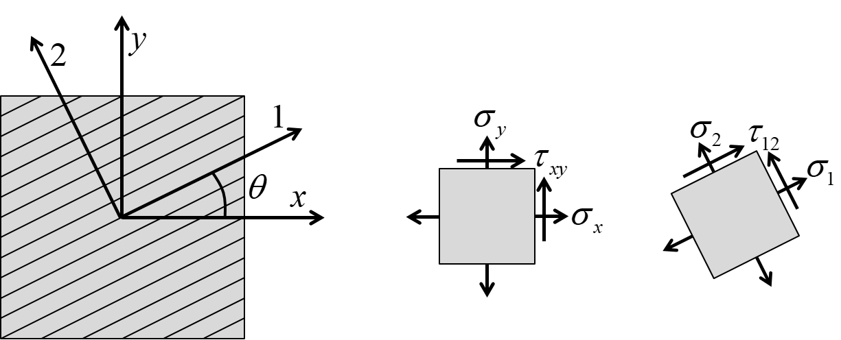
Figure-1: Definition of rotation about the z axis
Transformations of stresses, strains and elastic properties are fundamentally rotations of tensors. While any rotation could be relevant, one specific type of rotation is essential for composite engineering: the rotation about the normal to a plane (such as the laminate plane). This normal is commonly defined as the $z$-axis or the $3$-axis as illustrated in Figure-1. Note that the rotation is counterclockwise about the z-axis in a right-handed coordinate system.
Notation
$\boldsymbol{\sigma}, \boldsymbol{\varepsilon}, \mathbf{C}, \mathbf{S}$: Stress, strain, stiffness and compliance matrix in the material coordinate system ($1,2,3$).
$\boldsymbol{\sigma}', \boldsymbol{\varepsilon}', \mathbf{C}', \mathbf{S}'$: Stress, strain, stiffness and compliance matrix in the global coordinate system ($x,y,z$).
Rotation of coordinates
Transformation of coordinates $e_i$ from a system $x,y,z$ to a system $1,2,3$ is expressed by:
\begin{equation} \begin{bmatrix} e_1 \\ e_2 \\ e_3 \end{bmatrix}= \mathbf{R} \begin{bmatrix} e_x \\ e_y \\ e_z \end{bmatrix} \tag{1} \end{equation}where $\mathbf{R}$ is the rotation matrix. This rotation matrix may operate on all axis for a general rotation. For a rotation about the $z$-axis only, the rotation matrix is given by:
\begin{equation} \mathbf{R}= \begin{bmatrix} c & -s & 0 \\ s & c & 0 \\ 0 & 0 & 1 \end{bmatrix} \tag{2} \end{equation}where $c=\text{cos}(\theta)$ and $s=\text{sin}(\theta)$.
The details about general rotations are well described in this Wikipedia article.
Stress transformation
When $\mathbf{R}$ is the rotation matrix for a tranformation from the $x,y,z$ system to the $1,2,3$ system, the rotation of the stress tensor is given by:
\begin{equation} \boldsymbol{\sigma}=\mathbf{R}^{T}\boldsymbol{\sigma}'\mathbf{R} \tag{3} \end{equation}For at rotation $\theta$ about the z-axis, the details are:
\begin{equation} \begin{bmatrix} \sigma_{1} & \tau_{12} & \tau_{13} \\ \tau_{12} & \sigma_{2} & \tau_{23} \\ \tau_{13} & \tau_{23} & \sigma_{3} \end{bmatrix}= \begin{bmatrix} c & s & 0 \\ -s & c & 0 \\ 0 & 0 & 1 \end{bmatrix} \begin{bmatrix} \sigma_{x} & \tau_{xy} & \tau_{xz} \\ \tau_{xy} & \sigma_{y} & \tau_{yz} \\ \tau_{xz} & \tau_{yz} & \sigma_{z} \end{bmatrix} \begin{bmatrix} c & -s & 0 \\ s & c & 0 \\ 0 & 0 & 1 \end{bmatrix} \tag{4} \end{equation}The matrix notation is obtained by performing the right hand side matrix multiplications and arranging the system of equation as:
\begin{equation} \begin{bmatrix} \sigma_1 \\ \sigma_2 \\ \sigma_3 \\ \tau_{23} \\ \tau_{13} \\ \tau_{12} \end{bmatrix}= \begin{bmatrix} c^2 & s^2 & 0 & 0 & 0 & 2cs \\ s^2 & c^2 & 0 & 0 & 0 & -2cs \\ 0 & 0 & 1 & 0 & 0 & 0 \\ 0 & 0 & 0 & c & -s & 0 \\ 0 & 0 & 0 & s & c & 0 \\ -cs & cs & 0 & 0 & 0 & c^2-s^2 \end{bmatrix} \begin{bmatrix} \sigma_x \\ \sigma_y \\ \sigma_z \\ \tau_{yz} \\ \tau_{xz} \\ \tau_{xy} \end{bmatrix} \tag{5} \end{equation}The short notation is
\begin{equation} \boldsymbol{\sigma}= \mathbf{T}_{\sigma z} \boldsymbol{\sigma}' \tag{6} \end{equation}where the transformation matrix for stress is:
\begin{equation} \mathbf{T}_{\sigma z}= \begin{bmatrix} c^2 & s^2 & 0 & 0 & 0 & 2cs \\ s^2 & c^2 & 0 & 0 & 0 & -2cs \\ 0 & 0 & 1 & 0 & 0 & 0 \\ 0 & 0 & 0 & c & -s & 0 \\ 0 & 0 & 0 & s & c & 0 \\ -cs & cs & 0 & 0 & 0 & c^2-s^2 \end{bmatrix} \tag{7} \end{equation}Numerical implementation
The following function for the transformation matrix for stress takes a rotation angle (degrees) as the only argument, and returns the transformation matrix as a NumPy array:
import numpy as np

def T3Dsz(rot):
    rot=np.radians(rot)
    c=np.cos(rot)
    s=np.sin(rot)
    return    np.array([[ c*c ,  s*s ,  0.0 , 0.0 , 0.0  ,  2*c*s ],
                        [ s*s ,  c*c ,  0.0 , 0.0 , 0.0  , -2*c*s ],
                        [ 0.0 ,  0.0 ,  1.0 , 0.0 , 0.0  ,    0.0 ],
                        [ 0.0 ,  0.0 ,  0.0 ,   c ,  -s  ,    0.0 ],
                        [ 0.0 ,  0.0 ,  0.0 ,   s ,   c  ,    0.0 ],
                        [-c*s ,  c*s ,  0.0 , 0.0 , 0.0  ,c*c-s*s ]],
                        float)
Examples
Find the stress in a coordinate system rotated 45 degrees about the z-axis when the global stress is
$$\boldsymbol{\sigma}'= \begin{bmatrix} 100 & 0 & 0 & 0 & 0 & 0 \end{bmatrix}^T$$stress_xyz=(100,0,0,0,0,0)
Ts=T3Dsz(45)
stress_123=np.dot(Ts,stress_xyz)
print('Transformation matrix from T3Ds(angle) where angle=45 degrees:')
print()
print(np.array2string(Ts, precision=3, suppress_small=True, separator=' ', floatmode='maxprec') )
print()
print('Stress in local coordinate system is:')
print()
print(stress_123)
The stress in the global coordinate system is
$$\boldsymbol{\sigma}'= \begin{bmatrix} 100 & 0 & 0 & 0 & 0 & 0 \end{bmatrix}^T$$Illustrate how the stress components in a rotated coordinate system vary with the rotation angle:
s_xyz=(100,0,0,0,0,0)
a=np.linspace(0,90,91)
s11,s22,s12=[],[],[]
for angle in a:
    s_123=np.dot(T3Dsz(angle),s_xyz)
    s11.append(s_123[0])
    s22.append(s_123[1])
    s12.append(s_123[5])
import matplotlib.pyplot as plt
%matplotlib inline
fig,ax=plt.subplots(figsize=(5,3))
ax.plot(a,s11,color='red', label='$\sigma_1$')
ax.plot(a,s22,color='blue', label='$\sigma_2$')
ax.plot(a,s12,color='green', label=r'$\tau_{12}$')
ax.set_xlim(0,90)
ax.legend(loc='best')
ax.grid(True)
plt.show()

Verify that the transformation by the tensor notation and the transformation by the matrix notation give identical results:
import numpy as np

def convertToVectorform(tensor):
    return np.array([tensor[0,0],tensor[1,1],tensor[2,2],tensor[1,2],tensor[0,2],tensor[0,1]])

def convertToTensorform(vector):
    return np.array([ [vector[0] , vector[5] , vector[4]],
                      [vector[5] , vector[1] , vector[3]],
                      [vector[4] , vector[3] , vector[2]]])


# Generate a random state of stress (vector form):
stressV=-100+200*np.random.random(6)

# Converting the stress to tensor form:
stressT=convertToTensorform(stressV)

# A random angle between -90 and 90 degrees:
a=-90+90*np.random.random()

# The rotation matrix for z-axis rotation:
def RotationMatrix(angle):
    c=np.cos(np.radians(angle))
    s=np.sin(np.radians(angle))
    return    np.array([[ c, -s, 0],
                        [ s,  c, 0],
                        [ 0,  0, 1]])
R=RotationMatrix(a)

# Matrix notation result:
resultV=np.dot( T3Dsz(a) , stressV )
print('This one:')
print(np.array2string(resultV, precision=3, suppress_small=True, separator='  ', floatmode='maxprec') )

# Tensor notation result, converted to matrix notation:
resultT=np.dot( np.linalg.inv(R), np.dot(stressT,R)    )
resultV2=convertToVectorform(resultT)
print('should be equal to this one:')
print(np.array2string(resultV2, precision=3, suppress_small=True, separator='  ', floatmode='maxprec') )
Strain transformation
Transformation of the strain tensor follows the same rule as the transformation of the stress tensor:
\begin{equation} \boldsymbol{\varepsilon}=\mathbf{R}^{T}\boldsymbol{\varepsilon}'\mathbf{R} \tag{8} \end{equation}For a rotation about the $z$-axis:
\begin{equation} \begin{bmatrix} \varepsilon_{1} & \frac{1}{2}\gamma_{12} & \frac{1}{2}\gamma_{13} \\ \frac{1}{2}\gamma_{12} & \varepsilon_{2} & \frac{1}{2}\gamma_{23} \\ \frac{1}{2}\gamma_{13} & \frac{1}{2}\gamma_{23} & \varepsilon_{3} \end{bmatrix}= \begin{bmatrix} c & s & 0 \\ -s & c & 0 \\ 0 & 0 & 1 \end{bmatrix} \begin{bmatrix} \varepsilon_{x} & \frac{1}{2}\gamma_{xy} & \frac{1}{2}\gamma_{xz} \\ \frac{1}{2}\gamma_{xy} & \varepsilon_{y} & \frac{1}{2}\gamma_{yz} \\ \frac{1}{2}\gamma_{xz} & \frac{1}{2}\gamma_{yz} & \varepsilon_{z} \end{bmatrix} \begin{bmatrix} c & -s & 0 \\ s & c & 0 \\ 0 & 0 & 1 \end{bmatrix} \tag{9} \end{equation}The matrix notation is found by performing the operations and rearranging the system of equations:
\begin{equation} \begin{bmatrix} \varepsilon_1 \\ \varepsilon_2 \\ \varepsilon_3 \\ \gamma_{23} \\ \gamma_{13} \\ \gamma_{12} \end{bmatrix}= \begin{bmatrix} c^2 & s^2 & 0 & 0 & 0 & cs \\ s^2 & c^2 & 0 & 0 & 0 & -cs \\ 0 & 0 & 1 & 0 & 0 & 0 \\ 0 & 0 & 0 & c & -s & 0 \\ 0 & 0 & 0 & s & c & 0 \\ -2cs & 2cs & 0 & 0 & 0 & c^2-s^2 \end{bmatrix} \begin{bmatrix} \varepsilon_x \\ \varepsilon_y \\ \varepsilon_z \\ \gamma_{yz} \\ \gamma_{xz} \\ \gamma_{xy} \end{bmatrix} \tag{10} \end{equation}Short notation:
\begin{equation} \boldsymbol{\varepsilon}= \mathbf{T}_{\varepsilon z} \boldsymbol{\varepsilon}' \tag{11} \end{equation}where the transformation matrix for strain is:
\begin{equation} \mathbf{T}_{\epsilon z}= \begin{bmatrix} c^2 & s^2 & 0 & 0 & 0 & cs \\ s^2 & c^2 & 0 & 0 & 0 & -cs \\ 0 & 0 & 1 & 0 & 0 & 0 \\ 0 & 0 & 0 & c & -s & 0 \\ 0 & 0 & 0 & s & c & 0 \\ -2cs & 2cs & 0 & 0 & 0 & c^2-s^2 \end{bmatrix} \tag{12} \end{equation}Numerical implementaion:
def T3Dez(rot):
    rot=np.radians(rot)
    c=np.cos(rot)
    s=np.sin(rot)
    return    np.array([[ c*c ,  s*s ,  0.0 , 0.0 , 0.0  ,    c*s ],
                        [ s*s ,  c*c ,  0.0 , 0.0 , 0.0  ,   -c*s ],
                        [ 0.0 ,  0.0 ,  1.0 , 0.0 , 0.0  ,    0.0 ],
                        [ 0.0 ,  0.0 ,  0.0 ,   c ,  -s  ,    0.0 ],
                        [ 0.0 ,  0.0 ,  0.0 ,   s ,   c  ,    0.0 ],
                        [-2*c*s, 2*c*s, 0.0 , 0.0 , 0.0  ,c*c-s*s ]],
                        float)
Transformation of stiffness and compliance matrices
From Hooke's law: \begin{equation}\boldsymbol{\sigma} =\mathbf{C}\boldsymbol{\varepsilon} \tag{13} \end{equation}
Substituting the stress and strain using $\boldsymbol{\sigma}=\mathbf{T}_{\sigma z}\boldsymbol{\sigma}'$ and $\boldsymbol{\varepsilon}=\mathbf{T}_{\varepsilon z}\boldsymbol{\varepsilon}'$:
\begin{equation}\mathbf{T}_{\sigma z}\boldsymbol{\sigma}' =\mathbf{C} \mathbf{T}_{\varepsilon z} \boldsymbol{\varepsilon}' \tag{14} \end{equation}such that
\begin{equation} \boldsymbol{\sigma}' = \mathbf{T}_{\sigma z}^{-1} \mathbf{C} \mathbf{T}_{\varepsilon z} \boldsymbol{\varepsilon}' \tag{15} \end{equation}Hooke's law in the global coordinate system is:
\begin{equation} \boldsymbol{\sigma}' = \mathbf{C}' \boldsymbol{\varepsilon}' \tag{16} \end{equation}and therefore, the transformed stiffness matrix becomes:
\begin{equation} \mathbf{C{'}} = \mathbf{T}_{\sigma z}^{-1}\mathbf{C} \mathbf{T}_{\epsilon z} \tag{17} \end{equation}The compliance matrix in the global system is the inverse of the stiffness matrix:
\begin{equation} \mathbf{S{'}} = \mathbf{C}^{-1} \tag{18} \end{equation}Numerical implementaion
Functions from previously implemented code:
from compositelib import C3D
Creating a function for the transformation of the stiffness matrix:
def C3Dtz(C,rot):
    return np.dot(np.linalg.inv(T3Dsz(rot)), np.dot(C,T3Dez(rot)))
Example
import matlib

material1=matlib.newMaterial(E1=150000, E2=20000, E3=10000, v12=0.3, v13=0.4, v23=0.5, G12=5000, G13=4000, G23=3000)

C=C3D(material1)
Ct=C3Dtz(C,30)
print(np.array2string(Ct, precision=0, suppress_small=True, separator='  ', floatmode='maxprec') )
Find the strains in the global coordinate system for the previous case (30 degree orientation of the material) when the stress in the global coordinate system is
$$\boldsymbol{\sigma}'= \begin{bmatrix} 100 & 0 & 0 & 0 & 0 & 0 \end{bmatrix}^T$$s_xyz=(100,0,0,0,0,0)
St=np.linalg.inv(Ct)
e_xyz=np.dot(St, s_xyz)
print(np.array2string(e_xyz, precision=5, suppress_small=True, separator=' ', floatmode='maxprec') )
Illustration:
from plotlib import illustrateStrains
ex =  e_xyz[0]
ey =  e_xyz[1]
exy=  e_xyz[5]

illustrateStrains(ex, ey, exy, scaleFactor=100)

The connection between transformation and principal stresses is illustrated in the case study Principal stresses and transformations
General transformation
Counterclockwise rotations of stresses and strains about all axes as individual functions:
# Stress transformation

# About x-axis
def T3Dsx(rot):
    rot=np.radians(rot)
    c,s=np.cos(rot),np.sin(rot)
    return    np.array([[ 1.0 ,  0.0 ,  0.0 ,  0.0   , 0.0  , 0.0 ],
                        [ 0.0 ,  c*c ,  s*s ,  2*c*s , 0.0  , 0.0 ],
                        [ 0.0 ,  s*s ,  c*c , -2*c*s , 0.0  , 0.0 ],
                        [ 0.0 , -c*s ,  c*s ,c*c-s*s , 0.0  , 0.0 ],
                        [ 0.0 ,  0.0 ,  0.0 ,    0.0 ,   c  ,  -s ],
                        [ 0.0 ,  0.0 ,  0.0 ,    0.0 ,   s  ,   c ]],
                        float)


# About y-axis
def T3Dsy(rot):
    rot=np.radians(rot)
    c,s=np.cos(rot),np.sin(rot)
    return    np.array([[ c*c ,  0.0 ,  s*s , 0.0 , -2*c*s  , 0.0 ],
                        [ 0.0 ,  1.0 ,  0.0 , 0.0 ,    0.0  , 0.0 ],
                        [ s*s ,  0.0 ,  c*c , 0.0 ,  2*c*s  , 0.0 ],
                        [ 0.0 ,  0.0 ,  0.0 ,   c ,    0.0  ,   s ],
                        [ c*s ,  0.0 , -c*s , 0.0 ,c*c-s*s  , 0.0 ],
                        [ 0.0 ,  0.0 ,  0.0 ,  -s ,    0.0  ,   c ]],
                        float)

# About z-axis
def T3Dsz(rot):
    rot=np.radians(rot)
    c,s=np.cos(rot),np.sin(rot)
    return    np.array([[ c*c ,  s*s ,  0.0 , 0.0 , 0.0  ,  2*c*s ],
                        [ s*s ,  c*c ,  0.0 , 0.0 , 0.0  , -2*c*s ],
                        [ 0.0 ,  0.0 ,  1.0 , 0.0 , 0.0  ,    0.0 ],
                        [ 0.0 ,  0.0 ,  0.0 ,   c ,  -s  ,    0.0 ],
                        [ 0.0 ,  0.0 ,  0.0 ,   s ,   c  ,    0.0 ],
                        [-c*s ,  c*s ,  0.0 , 0.0 , 0.0  ,c*c-s*s ]],
                        float)


# Strain transformation

# About x-axis
def T3Dex(rot):
    rot=np.radians(rot)
    c,s=np.cos(rot),np.sin(rot)
    return    np.array([[ 1.0 ,   0.0 ,   0.0 ,    0.0 , 0.0  , 0.0 ],
                        [ 0.0 ,   c*c ,   s*s ,    c*s , 0.0  , 0.0 ],
                        [ 0.0 ,   s*s ,   c*c ,   -c*s , 0.0  , 0.0 ],
                        [ 0.0 ,-2*c*s , 2*c*s ,c*c-s*s , 0.0  , 0.0 ],
                        [ 0.0 ,   0.0 ,   0.0 ,    0.0 ,   c  ,  -s ],
                        [ 0.0 ,   0.0 ,   0.0 ,    0.0 ,   s  ,   c ]],
                        float)

# About y-axis
def T3Dey(rot):
    rot=np.radians(rot)
    c,s=np.cos(rot),np.sin(rot)
    return    np.array([[   c*c ,  0.0 ,   s*s , 0.0 ,   -c*s , 0.0 ],
                        [   0.0 ,  1.0 ,   0.0 , 0.0 ,    0.0 , 0.0 ],
                        [   s*s ,  0.0 ,   c*c , 0.0 ,    c*s , 0.0 ],
                        [   0.0 ,  0.0 ,   0.0 ,   c ,    0.0 ,   s ],
                        [ 2*c*s ,  0.0 , -2*c*s, 0.0 ,c*c-s*s , 0.0 ],
                        [   0.0 ,  0.0 ,   0.0 ,  -s ,    0.0 ,   c ]],
                        float)

# About z-axis
def T3Dez(rot):
    rot=np.radians(rot)
    c,s=np.cos(rot),np.sin(rot)
    return    np.array([[ c*c ,  s*s ,  0.0 , 0.0 , 0.0  ,    c*s ],
                        [ s*s ,  c*c ,  0.0 , 0.0 , 0.0  ,   -c*s ],
                        [ 0.0 ,  0.0 ,  1.0 , 0.0 , 0.0  ,    0.0 ],
                        [ 0.0 ,  0.0 ,  0.0 ,   c ,  -s  ,    0.0 ],
                        [ 0.0 ,  0.0 ,  0.0 ,   s ,   c  ,    0.0 ],
                        [-2*c*s, 2*c*s, 0.0 , 0.0 , 0.0  ,c*c-s*s ]],
                        float)


