In [ ]:
from abaqus import *
from abaqusConstants import *
from custom.... import...

def generic_useful_function(parameters):
    # generic tool
    ...

def create_submit_results(modelname, par1, par2, ...):
    # Establish parameter relations
    # Parts, properties and mesh
    # Assembly and interactions
    # Steps and loading
    # Job and results
    ...

# Optional:

def optimization_or_parameter_study():
    # Initial conditions and decission criteria
    doLoop:
        createSubmitAndResults(modelname, par1, par2, ...)
        # Make decissions
        ...
Example: A finite length cylinder subjected to internal pressure
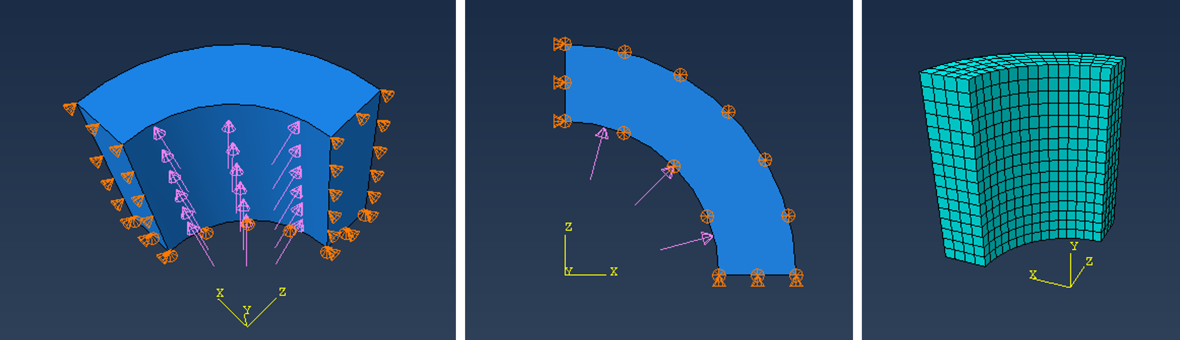
A finite length, thick walled steel sylinder shall be subjected to internal pressure. The cylinder is open in both ends, and symmetry can be assumed about all three pricipal planes.
The scipt has two functions:
cylinder(modelname, L, ri, ro, esize, P)which creates a new model based on the parameters in the argument, submits the job and returns the global element size, the number of elements and the maximum value of the von mises stress.doLoop_meshConvergency()is a wrapper that runs a number of models where the element size is gradualy decreasing, everything else being identical. The function completes by printing lists of the relevant parameters:
In [ ]:
from abaqus import *
from abaqusConstants import *
from customtools import getByPO, getByR

def cylinder(modelname, L, ri, ro, esize, P):
    mod = mdb.Model(name=modelname)
    ske = mod.ConstrainedSketch(name='__profile__', sheetSize=200.0)
    ske.ConstructionLine(point1=(0.0, -100.0), point2=(0.0, 100.0))
    ske.rectangle(point1=(ri, 0.0), point2=(ro, L))
    prt = mod.Part(name='P1', dimensionality=THREE_D, type=DEFORMABLE_BODY)
    prt.BaseSolidRevolve(sketch=ske, angle=90.0, flipRevolveDirection=OFF)
    del ske
    session.viewports['Viewport: 1'].setValues(displayedObject=prt)

    # Sets and surface:

    prt.Set(name='cells all', cells = prt.cells)
    prt.Set(name='face xsym', faces=getByPO(prt.faces,x=0))
    prt.Set(name='face ysym', faces=getByPO(prt.faces,y=0))
    prt.Set(name='face zsym', faces=getByPO(prt.faces,z=0))
    prt.Surface(name='surface inner', side1Faces = getByR(prt.faces,r=ri))

    # Material, section and mesh

    mat = mod.Material(name='Steel')
    mat.Elastic(table=((200000.0, 0.3), ))
    mod.HomogeneousSolidSection(name='Section-1', material='Steel', thickness=None)
    prt.SectionAssignment(region=prt.sets['cells all'], sectionName='Section-1')
    prt.seedPart(size=esize, deviationFactor=0.1, minSizeFactor=0.1)
    prt.generateMesh()

    # Assembly, step and loading

    ass = mod.rootAssembly
    ass.DatumCsysByDefault(CARTESIAN)
    ins = ass.Instance(name='P1', part=prt, dependent=ON)
    mod.DisplacementBC(name='BC-XSYM', createStepName='Initial', region=ins.sets['face xsym'], u1=SET)
    mod.DisplacementBC(name='BC-YSYM', createStepName='Initial', region=ins.sets['face ysym'], u2=SET)
    mod.DisplacementBC(name='BC-ZSYM', createStepName='Initial', region=ins.sets['face zsym'], u3=SET)
    mod.StaticStep(name='Step-1', previous='Initial')
    mod.Pressure(name='Pressure', createStepName='Step-1', region=ins.surfaces['surface inner'], magnitude=P)

    # Job and result

    job = mdb.Job(name=modelname, model=modelname)
    job.submit(consistencyChecking=OFF)
    job.waitForCompletion()
    odb = session.openOdb(name=modelname+'.odb')
    mises = [value.data for value in odb.steps['Step-1'].frames[-1].fieldOutputs['S'].getScalarField(MISES).values]

    return esize, len(prt.elements), max(mises)


def doLoop_meshConvergency():
    esizeList, noelList, maxmisesList = [], [], []
    esize = 20.0
    for i in range(0,10):
        esize, noel, maxmises = cylinder(modelname='M-'+str(i), L=100.0, ri=50.0, ro=75.0, esize=esize, P=100.0)
        esizeList.append(round(esize,3))
        noelList.append(noel)
        maxmisesList.append(round(maxmises,1))
        esize=0.75*esize
    print esizeList
    print noelList
    print maxmisesList

doLoop_meshConvergency()
The printout from the script with the parameters as above is three lists, copied to this notebook:
In [11]:
esize = [20.0, 15.0, 11.25, 8.438, 6.328, 4.746, 3.56, 2.67, 2.002, 1.502]
noel  = [25, 70, 126, 396, 960, 2205, 5292, 11988, 29400, 74035]
mises = [222.7, 261.9, 261.9, 278.9, 288.4, 294.5, 301.8, 306.0, 309.8, 313.2]
In this case, the inverse element size on the x-axis of a plot, makes a useful illustration on how the maximum mises stress increases with finer mesh. Employing matplotlib:
In [12]:
inv_esize = [1/es for es in esize]
import matplotlib.pyplot as plt
plt.figure(figsize=(6,2))
plt.plot(inv_esize, mises)
plt.grid()
plt.show()


