Flexural testing¶

A FEA model replicating a flexural test, such as the 3-point bending test, is very useful for interpretation of test results. While simple configurations and homogeneous test specimen can be analyzed using analytical solutions, this may not be the case for laminated specimen with complex behaviors.

Model-1¶

The script was built partly on the script in Shell laminate where the process is recorded in the video Flexural testing Part-1

Key features¶

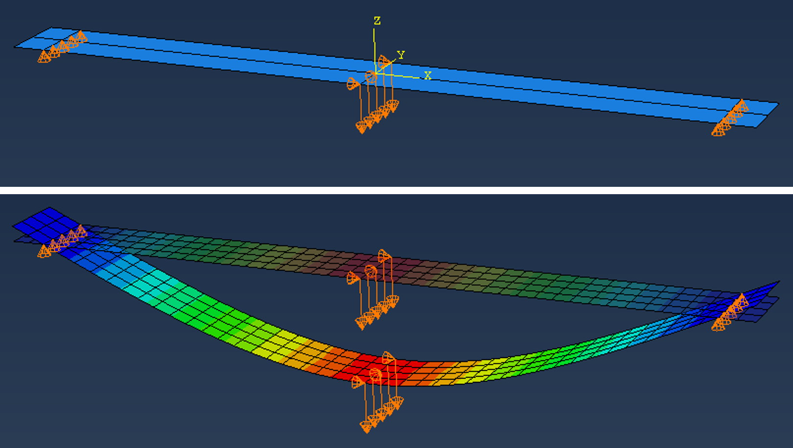
The test specimen is shell-based (S4R) with a composite layup
Supports and loading are modeled using simple boundary conditions and prescribed displacement
The model allows for both linear solution and non-linear solution due to large deformation by the argument nonlin=False or nonlin=True

from abaqus import *
from abaqusConstants import *
import regionToolset

def matlib(modelname):
    mod = mdb.models[modelname]
    mat = mod.Material('E-glass/Epoxy')
    mat.Density(table=((2000e-12, ), ))
    mat.Elastic(type=ENGINEERING_CONSTANTS, 
        table=((40000, 10000, 10000, 0.3, 0.3, 0.3, 3800, 3800, 3400,), ))
    mat.Expansion(type=ORTHOTROPIC, table=((7E-06, 22E-06, 22E-06), ))

lam1 = [{'mat':'E-glass/Epoxy', 'ori':   0, 'thi': 1.0},
        {'mat':'E-glass/Epoxy', 'ori':  90, 'thi': 1.0},
        {'mat':'E-glass/Epoxy', 'ori':  90, 'thi': 1.0},
        {'mat':'E-glass/Epoxy', 'ori':   0, 'thi': 1.0}]

def flex3pShell(modelname, L, b, dL, laminate, esize, U3, nonlin, dts):
    
    t = sum([layer['thi'] for layer in laminate])

    # new model:
    mod = mdb.Model(name=modelname)

    # materials and sections:
    matlib(modelname)
    for matname in mod.materials.keys():
        mod.HomogeneousSolidSection(name=matname, material=matname, thickness=None)
     
    # planar shell:   
    ske = mod.ConstrainedSketch(name='__profile__', sheetSize=200.0)
    ske.rectangle(point1=(0.0, 0.0), point2=(L+2*dL, b))
    prt = mod.Part(name='Specimen', dimensionality=THREE_D, type=DEFORMABLE_BODY)
    prt.BaseShell(sketch=ske)
    del mod.sketches['__profile__']
    session.viewports['Viewport: 1'].setValues(displayedObject=prt)

    # Partitions:
    id=prt.DatumPlaneByPrincipalPlane(principalPlane=XZPLANE, offset=b/2.0).id
    prt.PartitionFaceByDatumPlane(datumPlane=prt.datums[id], faces=prt.faces)    
    for xpos in [dL, dL+L/2.0, dL+L]:
        id=prt.DatumPlaneByPrincipalPlane(principalPlane=YZPLANE, offset=xpos).id
        prt.PartitionFaceByDatumPlane(datumPlane=prt.datums[id], faces=prt.faces)

    # layup:
    id = prt.DatumCsysByDefault(coordSysType=CARTESIAN).id
    layupOrientation = prt.datums[id]
    region = regionToolset.Region(faces=prt.faces)
    compositeLayup = prt.CompositeLayup(name='Layup1', elementType=SHELL, offsetType=MIDDLE_SURFACE)
    compositeLayup.Section()
    compositeLayup.ReferenceOrientation(orientationType=SYSTEM, localCsys=layupOrientation, axis=AXIS_3)
    count = 1
    for layer in laminate:
        compositeLayup.CompositePly(suppressed=False, plyName='Ply-'+str(count), region=region, 
            material=layer['mat'], thicknessType=SPECIFY_THICKNESS, thickness=layer['thi'], 
            orientationType=SPECIFY_ORIENT, orientationValue=layer['ori'] )
        count = count + 1

    # Mesh:
    prt.seedPart(size=esize, deviationFactor=0.1, minSizeFactor=0.1)
    prt.generateMesh()

    # Assembly:
    ass = mod.rootAssembly
    ass.DatumCsysByDefault(CARTESIAN)
    ins = ass.Instance(name='Specimen', part=prt, dependent=ON)
    ass.translate(instanceList=('Specimen', ), vector=(-L/2.0-dL, -b/2.0, 0.0))

    # Boundary conditions:
    edges = ins.edges.findAt(((-L/2.0, -b/4.0, 0.0), ), ((-L/2.0, b/4.0, 0.0), ), 
        ((L/2.0, -b/4.0, 0.0), ), ((L/2.0, b/4.0, 0.0), ))
    region = ass.Set(edges=edges, name='EDGES-SUPPORT')
    mod.DisplacementBC(name='BC-SUPPORT', createStepName='Initial', region=region, u3=SET)
    edges = ins.edges.findAt(((0.0, -b/4.0, 0.0), ), ((0.0, b/4.0, 0.0), ))
    region = ass.Set(edges=edges, name='EDGES-LOADING')
    mod.DisplacementBC(name='BC-LOADING', createStepName='Initial', region=region, u3=SET )
    
    verts = ins.vertices.findAt(((0.0, -b/2.0, 0.0), ), ((0.0, b/2, 0.0), ))
    region = ass.Set(vertices=verts, name='VERTICES-RB1')
    mod.DisplacementBC(name='BC-RB1', createStepName='Initial', region=region, u1=SET)
    verts = ins.vertices.findAt(((0.0, 0.0, 0.0), ))
    region = ass.Set(vertices=verts, name='VERTICES-RB2')
    mod.DisplacementBC(name='BC-RB2', createStepName='Initial', region=region, u2=SET)
    
    # Step and loading
    if nonlin:
        mod.StaticStep(name='Step-1', previous='Initial', initialInc=dts, maxInc=dts, nlgeom=ON)
    else:
        mod.StaticStep(name='Step-1', previous='Initial')
    mod.boundaryConditions['BC-LOADING'].setValuesInStep(stepName='Step-1', u3=-U3)
    
    # Job and results
    job=mdb.Job(name=modelname, model=modelname)
    job.submit(consistencyChecking=OFF)
    job.waitForCompletion()
    odb = session.openOdb(name=modelname+'.odb')
    session.viewports['Viewport: 1'].setValues(displayedObject=odb)
    session.viewports['Viewport: 1'].makeCurrent()

    # displacement and sum of reaction force
    uz = []
    fz = []
    region = odb.rootAssembly.nodeSets['EDGES-LOADING']
    for frame in odb.steps['Step-1'].frames:
        rfs = frame.fieldOutputs['RF'].getSubset(region = region).values
        us = frame.fieldOutputs['U'].getSubset(region = region).values
        rfsum = sum([rf.data[2] for rf in rfs])
        u = us[0].data[2]
        uz.append(-u)         # reversed sign
        fz.append(-rfsum)     # reversed sign

    print 'uz=', uz
    print 'fz=', fz

Example¶

flex3pShell(modelname='Beam-1', L=200, b=20, dL=10, laminate=lam1, esize=5, U3=30, nonlin=False, dts=1.0)
flex3pShell(modelname='Beam-2', L=200, b=20, dL=10, laminate=lam1, esize=5, U3=30, nonlin=True,  dts=0.1)

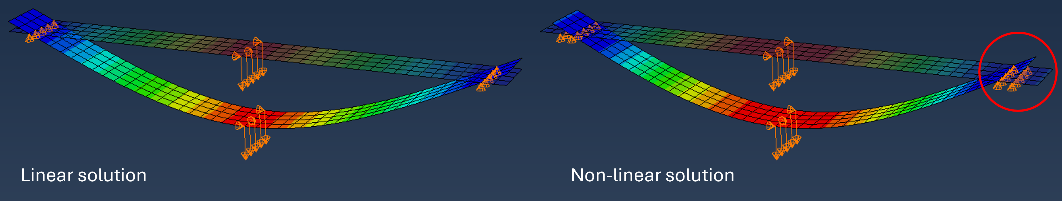
The laminate and the material is as given in the script above, and the only difference between the two models is linear versus non-linear solution.

Observe how the bounday conditions for the supports moves along the x-direction in the non-linear solution. This effect has obvously consequences for the load versus deflection results.

Results from the script:

uz_1 = [0.0, 30.0]
fz_1 = [0.0, 697.800720214844]

uz_2 = [0.0, 3.0, 6.0, 9.0, 12.0, 15.0, 18.0, 21.0, 24.0, 27.0, 30.0]
fz_2 = [0.0, 69.8445739746094, 140.07772064209, 211.095611572266, 283.311660766602, 357.165130615234, 
        433.131896972656, 511.736709594727, 593.568359375, 679.298034667969, 769.702789306641]

import matplotlib.pyplot as plt
plt.plot(uz_1,fz_1, label='Linear solution')
plt.plot(uz_2,fz_2, label='Non-linear solution')
plt.xlim(0,)
plt.ylim(0,)
plt.grid()
plt.legend()
plt.show()

Model-2¶

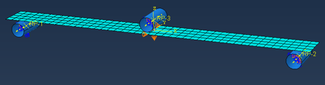
The simple boundary conditions for support and loading is now replaced with analytical rigid parts representing the cylinders (rollers) commonly used in this test configuration.

Note that this configuration is only meanigful when large deformation is presumed.

See the video Flexural testing Part-2 for details

from abaqus import *
from abaqusConstants import *
import regionToolset

def matlib(modelname):
    mod = mdb.models[modelname]
    mat = mod.Material('E-glass/Epoxy')
    mat.Density(table=((2000e-12, ), ))
    mat.Elastic(type=ENGINEERING_CONSTANTS, 
        table=((40000, 10000, 10000, 0.3, 0.3, 0.3, 3800, 3800, 3400,), ))
    mat.Expansion(type=ORTHOTROPIC, table=((7E-06, 22E-06, 22E-06), ))

lam1 = [{'mat':'E-glass/Epoxy', 'ori':   0, 'thi': 1.0},
        {'mat':'E-glass/Epoxy', 'ori':  90, 'thi': 1.0},
        {'mat':'E-glass/Epoxy', 'ori':  90, 'thi': 1.0},
        {'mat':'E-glass/Epoxy', 'ori':   0, 'thi': 1.0}]

def flex3pShellAR(modelname, L, b, dL, laminate, esize, r, U3, dts):
    
    t = sum([layer['thi'] for layer in laminate])

    # new model:
    mod = mdb.Model(name=modelname)

    # materials and sections:
    matlib(modelname)
    for matname in mod.materials.keys():
        mod.HomogeneousSolidSection(name=matname, material=matname, thickness=None)
     
    # planar shell:   
    ske = mod.ConstrainedSketch(name='__profile__', sheetSize=200.0)
    ske.rectangle(point1=(0.0, 0.0), point2=(L+2*dL, b))
    prt = mod.Part(name='Specimen', dimensionality=THREE_D, type=DEFORMABLE_BODY)
    prt.BaseShell(sketch=ske)
    del mod.sketches['__profile__']
    session.viewports['Viewport: 1'].setValues(displayedObject=prt)

    # Partitions:
    id=prt.DatumPlaneByPrincipalPlane(principalPlane=XZPLANE, offset=b/2.0).id
    prt.PartitionFaceByDatumPlane(datumPlane=prt.datums[id], faces=prt.faces)    
    for xpos in [dL+r, dL+L/2.0-r, dL+L/2.0, dL+L/2.0+r, dL+L-r]:
        id=prt.DatumPlaneByPrincipalPlane(principalPlane=YZPLANE, offset=xpos).id
        prt.PartitionFaceByDatumPlane(datumPlane=prt.datums[id], faces=prt.faces)

    # layup:
    id = prt.DatumCsysByDefault(coordSysType=CARTESIAN).id
    layupOrientation = prt.datums[id]
    region = regionToolset.Region(faces=prt.faces)
    compositeLayup = prt.CompositeLayup(name='Layup1', elementType=SHELL, offsetType=MIDDLE_SURFACE)
    compositeLayup.Section()
    compositeLayup.ReferenceOrientation(orientationType=SYSTEM, localCsys=layupOrientation, axis=AXIS_3)
    count = 1
    for layer in laminate:
        compositeLayup.CompositePly(suppressed=False, plyName='Ply-'+str(count), region=region, 
            material=layer['mat'], thicknessType=SPECIFY_THICKNESS, thickness=layer['thi'], 
            orientationType=SPECIFY_ORIENT, orientationValue=layer['ori'] )
        count = count + 1

    # Mesh:
    prt.seedPart(size=esize, deviationFactor=0.1, minSizeFactor=0.1)
    prt.generateMesh()

    # Assembly:
    ass = mod.rootAssembly
    ass.DatumCsysByDefault(CARTESIAN)
    ins = ass.Instance(name='Specimen', part=prt, dependent=ON)
    ass.translate(instanceList=('Specimen', ), vector=(-L/2.0-dL, -b/2.0, 0.0))

    # Rollers:
    ske = mod.ConstrainedSketch(name='__profile__', sheetSize=200.0)
    ske.ConstructionLine(point1=(0.0, -100.0), point2=(0.0, 100.0))
    ske.Line(point1=(r, -1.1*b/2.0), point2=(r, 1.1*b/2.0))
    prtr = mod.Part(name='Roller', dimensionality=THREE_D, type=ANALYTIC_RIGID_SURFACE)
    prtr.AnalyticRigidSurfRevolve(sketch=ske)
    del mod.sketches['__profile__']

    # Roller instances:
    insRL = ass.Instance(name='Roller-L', part=prtr, dependent=ON)
    ass.translate(instanceList=('Roller-L', ), vector=(-L/2.0, 0.0, -r-t/2.0))
    insRR = ass.Instance(name='Roller-R', part=prtr, dependent=ON)
    ass.translate(instanceList=('Roller-R', ), vector=(L/2.0, 0.0, -r-t/2.0))    
    insRC = ass.Instance(name='Roller-C', part=prtr, dependent=ON)
    ass.translate(instanceList=('Roller-C', ), vector=(0.0, 0.0, r+t/2.0))
    
    # Contact interactions:
    mod.ContactProperty('Contact-properties')
    region1=ass.Surface(side2Faces=insRL.faces, name='Surface-roller-L')
    region2=ass.Surface(side2Faces=ins.faces.getByBoundingBox(xMax=-L/2.0+r), name='Surface-L')
    mod.SurfaceToSurfaceContactStd(name='Contact-L', createStepName='Initial', main=region1, secondary=region2, 
        sliding=FINITE, thickness=ON, interactionProperty='Contact-properties', adjustMethod=NONE, 
        initialClearance=OMIT, datumAxis=None, clearanceRegion=None)
     
    region1=ass.Surface(side2Faces=insRR.faces, name='Surface-roller-R')
    region2=ass.Surface(side2Faces=ins.faces.getByBoundingBox(xMin=L/2.0-r), name='Surface-R')
    mod.SurfaceToSurfaceContactStd(name='Contact-R', createStepName='Initial', main=region1, secondary=region2, 
        sliding=FINITE, thickness=ON, interactionProperty='Contact-properties', adjustMethod=NONE, 
        initialClearance=OMIT, datumAxis=None, clearanceRegion=None)        

    region1=ass.Surface(side2Faces=insRC.faces, name='Surface-roller-C')
    region2=ass.Surface(side1Faces=ins.faces.getByBoundingBox(xMin=-r, xMax=r), name='Surface-C')
    mod.SurfaceToSurfaceContactStd(name='Contact-C', createStepName='Initial', main=region1, secondary=region2, 
        sliding=FINITE, thickness=ON, interactionProperty='Contact-properties', adjustMethod=NONE, 
        initialClearance=OMIT, datumAxis=None, clearanceRegion=None)      

    # Constraints and BC, rollers:
    id = ass.ReferencePoint(point=(-L/2.0, 0.0, -r-t/2.0)).id
    regionRPL = ass.Set(name='RPL', referencePoints = (ass.referencePoints[id],))
    regionRollerL = ass.surfaces['Surface-roller-L']
    mod.RigidBody(name='Constraint-Roller-L', refPointRegion=regionRPL, surfaceRegion=regionRollerL)
    mod.EncastreBC(name='BC-FIX-L', createStepName='Initial', region=regionRPL, localCsys=None)
    id = ass.ReferencePoint(point=(L/2.0, 0.0, -r-t/2.0)).id
    regionRPR = ass.Set(name='RPR', referencePoints = (ass.referencePoints[id],))
    regionRollerR = ass.surfaces['Surface-roller-R']
    mod.RigidBody(name='Constraint-Roller-R', refPointRegion=regionRPR, surfaceRegion=regionRollerR)
    mod.EncastreBC(name='BC-FIX-R', createStepName='Initial', region=regionRPR, localCsys=None)    
    id = ass.ReferencePoint(point=(0.0, 0.0, r+t/2.0)).id
    regionRPC = ass.Set(name='RPC', referencePoints = (ass.referencePoints[id],))
    regionRollerC = ass.surfaces['Surface-roller-C']
    mod.RigidBody(name='Constraint-Roller-C', refPointRegion=regionRPC, surfaceRegion=regionRollerC)
    mod.DisplacementBC(name='BC-C', createStepName='Initial', region=regionRPC, 
        u1=SET, u2=SET, u3=SET, ur1=SET, ur2=SET, ur3=SET, 
        amplitude=UNSET, distributionType=UNIFORM, fieldName='', localCsys=None)    

    # BC on specimen:
    verts = ins.vertices.findAt(((0.0, -b/2.0, 0.0), ), ((0.0, b/2, 0.0), ))
    region = ass.Set(vertices=verts, name='VERTICES-RB1')
    mod.DisplacementBC(name='BC-RB1', createStepName='Initial', region=region, u1=SET)
    verts = ins.vertices.findAt(((0.0, 0.0, 0.0), ))
    region = ass.Set(vertices=verts, name='VERTICES-RB2')
    mod.DisplacementBC(name='BC-RB2', createStepName='Initial', region=region, u2=SET)
    
    # Step and loading
    mod.StaticStep(name='Step-1', previous='Initial', initialInc=dts, maxInc=dts, nlgeom=ON)
    mod.boundaryConditions['BC-C'].setValuesInStep(stepName='Step-1', u3=-U3)
    
    # Job and results
    job=mdb.Job(name=modelname, model=modelname)
    job.submit(consistencyChecking=OFF)
    job.waitForCompletion()
    odb = session.openOdb(name=modelname+'.odb')
    session.viewports['Viewport: 1'].setValues(displayedObject=odb)
    session.viewports['Viewport: 1'].makeCurrent()

    # displacement and reaction force
    uz = []
    fz = []
    region = odb.rootAssembly.nodeSets['RPC']
    for frame in odb.steps['Step-1'].frames:
        rfs = frame.fieldOutputs['RF'].getSubset(region = region).values
        us = frame.fieldOutputs['U'].getSubset(region = region).values
        rf = rfs[0].data[2]
        u = us[0].data[2]
        uz.append(-u)      # reversed sign
        fz.append(-rf)     # reversed sign

    print 'uz=', uz
    print 'fz=', fz

Example¶

The test specimen is identical to the examples used in the script for Model-1:

flex3pShellAR(modelname='Beam-3', L=200, b=20, dL=10, laminate=lam1, esize=5, r=5, U3=30,  dts=0.1)

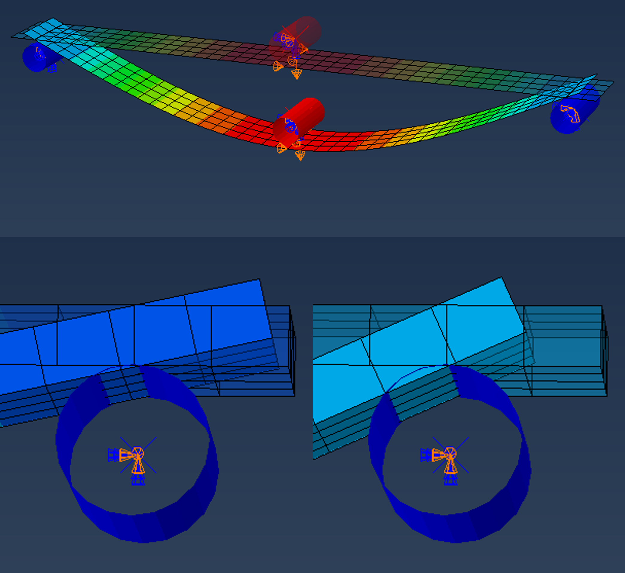
The radius of the rollers is 5 mm and by rendering the shell thickness we can observe that the rollers are partly penetrating the surfaces of the laminated specimen. This is an effect that will influence the accuracy of the results by introducing an added artificial compliance in the system.

Comparison of the results so far indicates that the effect of contact penetration occurs relatively early during the loading:

uz_3 = [0.0, 3.0, 6.0, 9.0, 12.0, 15.0, 18.0, 21.0, 24.0, 27.0, 30.0]
fz_3 = [0.0, 59.709198, 129.18138, 197.94868, 265.4801, 331.08167, 393.94067, 
        453.1642, 507.79984, 556.9399, 601.08484]

plt.plot(uz_1,fz_1, label='Linear solution')
plt.plot(uz_2,fz_2, label='Non-linear solution')
plt.plot(uz_3,fz_3, label='Analytical rigid rollers')
plt.xlim(0,)
plt.ylim(0,)
plt.grid()
plt.legend()
plt.show()

The challenge with contact penetration can be mittigated by reducing the element size:

flex3pShellAR(modelname='Beam-4', L=200, b=20, dL=10, laminate=lam1, esize=2, r=5, U3=30,  dts=0.1)

uz_4= [0.0, 0.75, 1.5, 2.625, 4.3125, 6.84375, 9.84375, 12.84375, 15.84375, 18.84375, 21.84375, 24.84375, 27.84375, 30.0]
fz_4= [0.0, 14.935997, 31.986013, 57.57044, 98.80254, 158.75449, 228.33217, 295.76395, 351.6792, 413.3955, 471.53235, 
       525.2242, 558.393, 591.8476]

plt.plot(uz_1,fz_1, label='Linear solution')
plt.plot(uz_2,fz_2, label='Non-linear solution')
plt.plot(uz_4,fz_4, label='Analytical rigid rollers, esize=2')
plt.xlim(0,)
plt.ylim(0,)
plt.grid()
plt.legend()
plt.show()

Observe that the time-stepping has been automatically changed (smaller time steps than 0.1 were needed by Abaqus).

Useful additions for layered shells¶

Include failure strength properties, for example a carbon fiber material.

(remember to change the material in the layup as well)

def matlib(modelname):
    mod = mdb.models[modelname]
    mat = mod.Material('Carbon/Epoxy(a)')
    mat.Density(table=((1600e-12, ), ))
    mat.Elastic(type=ENGINEERING_CONSTANTS, 
        table=((130000.0, 10000.0, 10000.0, 0.28, 0.28, 0.5, 4500.0, 4500.0, 3500.0,), ))
    mat.elastic.FailStress(table=((1800.0, 1200.0, 40.0, 180.0, 70.0, -0.5, 0.0), ))

Add field output request for the layup to include such as section forces and curvatures and failure indices (exposure factors)

Se Shell elements and laminate theory

The following entry must be placed before Job:

    # Field output request
    mod.FieldOutputRequest(name='F-Output-2', createStepName='Step-1', variables=('S', 'E', 'SE', 'SF', 'CFAILURE'), 
        layupNames=('Specimen.Layup1', ), layupLocationMethod=ALL_LOCATIONS, rebar=EXCLUDE)

Disclaimer:This site is designed for educational purposes only. There are most likely errors, mistakes, typos, and poorly crafted statements that are not detected yet... www.ntnu.edu/employees/nils.p.vedvik