Test methods
Tensile tests of unidirectional lamina
Uniaxial tensile tests are conducted on unidirectional laminae to determine the longitudinal and transverse Young's moduli $E_1$ and $E_2$, the Poisson's ratios $\nu_{12}$ and $\nu_{21}$ as well as the basic longitudinal and transverse strength parameters $X_T$ and $Y_T$.
Compressive tests of unidirectional lamina
The longitudinal compressive strength $X_C$ and the transverse compressive strength $Y_C$ are obtained by compressive tests of unidirectional lamina. Compression testing of composites is difficult because of the tendency for premature failure due to buckling. Techniques used to mitigate this problem are either based on a very short unsupported length, or some kind of support mechanisms (anti-buckling device).
Shear tests
There are several commonly used test methods for determining the shear modulus $G_{12}$ and the shear strength $S_{12}$:
- Tensile testing of symmetric [$\pm$45] laminates and back calculating the shear stress and shear strain
- Off-axis tensile testing: The testing is conducted on unidirectional laminae where the fiber orientation is oriented by a relatively small angel (about 10 degrees) relatively to the loading direction
- Torque on thin-wall tubular hoop-wound specimen
- Rail shear test
- Arcan test
- Iosipescu test.
Biaxial testing
Of the various methods that have been proposed, the tubular speciment appears to be the most versatile and offers the greatest potential. It offers the possibility of applying any desired biaxial state of stress by the the combination of axial load, internal or external pressure and torque.
Flexural testing
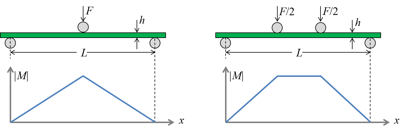
The two methods most usually used for the determination of flexural properties of laminates are the three-point and four-point tests.
Interlaminar fracture mechanical testing
Interlaminar crack propagation can occur in mode I, II and III corresponding to the fracture energies $G_{Ic}$, $G_{IIc}$ and $G_{IIIc}$. In TMM4175, the double cantilever beam (DCB) test for mode I, and the end-notch flexure (ENF) test for mode II will be discussed.
Tensile testing
Uniaxial tensile tests are conducted on unidirectional laminae to determine the longitudinal and transverse Young's moduli $E_1$ and $E_2$, the Poisson's ratios $\nu_{12}$ and $\nu_{21}$, the basic longitudinal and transverse strength parameters $X_T$ and $Y_T$ as well as coresponding failure strains.
The measurements of these properties is in theory very simple: A thin strip of a UD composite is placed into the grips of a mechanical testing machine and loaded slowly in tension. To determine the modulus of elasticity and Poisson’s ratio, strains are measured during the initial stage of the test, using strain gages as illustrated in Figure-1 and 2 or extensometers. Loading continues to ultimate failure, the point at which tensile strength and ultimate tensile strain are obtained.
In practice, however, obtaining valid results for strength parameters is not always easy.
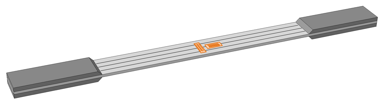
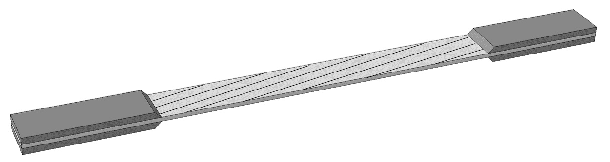
Figure-1: Tensile test specimen with tabs for longitudinal direction of UD laminae.
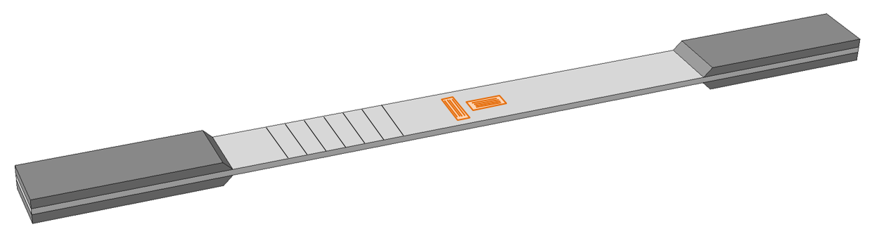
Figure-2: Tensile test specimen with tabs for transverse direction of UD laminae.
Generally, tensile specimen must be designed in such a way that stress during the test will be greater in the central test section than in the clamped regions at the end. For isotropic materials, the width of the specimen is gradually reduced from the ends into the central gauge length section, typically referred to as a “dog-bone” specimen. In the case of UD composites this is not an option since axial splitting of the specimen will occurs well before ultimate failure, effectively producing an untapered specimen. These axial cracks result from the relatively low shear strength of the UD composite material combined with relatively high shear stresses in these regions.
The solution for composites is usually to add bonded tabs on the ends. When a tabbed tensile specimen is tested, the load is transferred through shear at the gripped tab surfaces. The tabbing material and the adhesive bond must have shear strength adequate to transfer the load into the composite to produce failure while simultatneously prevent axial cracking and stress consentration. An effective means of minimizing the stress concentration is to use a carefully choosen taper angle as illustrated in Figure-1 and Figure-2.
Compression testing
Compressive testing of composites is notoriously difficult. The mode of failure involves a mixture of global column buckling of the entire specimen, to local micro buckling of the individual fibers. End loaded specimens tend to split from the ends and indirect loading by means of shear is often used. Shear loading introduces other challenges where failures often initiate at the grips due to stress concentration in this area. The test methods tend to underestimate the intrinsic compressive strength of the composites. Many axial compression test methods are some variation of the Celanese compression test described in ASTM D3410. In this method, a thin, straight-sided specimen with a small gauge length is loaded in the tabbed region using inverted cone wedge grips. The IITRI fixture shown below, which is a minor modification, incorporates flat wedge surfaces rather than conical surfaces for greater stability.

Tabs bonded to the specimen are recommended when testing unidirectional materials in the fiber direction. Transverse compression testing can however often be successfully conducted without tabs.
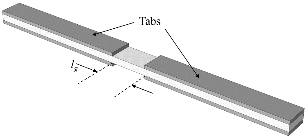
The ASTM D3410 Standard Test Method for Compressive Properties of Polymer Matrix Composite Materials with Unsupported Gage Section by Shear Loading specifies the combination of specimen dimensions with respect to various stiffnesses and expected failure strength. The required minimum thickness (h) for the unidirectional E-glass/Epoxy loaded in the fiber direction and having a gauge length lg is given by:
E1 = 40000
Xc = 700
G13 = 3800
lg = 15
h = lg/(0.9069*((1-1.2*Xc/G13)*(E1/Xc))**0.5)
print('Minimum thickness = ',h, 'mm')
In the above relation, Xc is the expected compressive strength. If the material data is based on anything but the maximum value obtained (such as mean, characteristic, etc), we should increase this value:
Xc = 1000
h = lg/(0.9069*((1-1.2*Xc/G13)*(E1/Xc))**0.5)
print('Minimum thickness = ',h, 'mm')
More on this test method in the case study Compression testing of UD composites
Shear testing
There is a greater variety of shear test methods origin from the fact that it is difficult to obtaining a reasonably pure and uniform shear stress state in small and simple test specimen. Hence, many shear test methods actually involve a mixed mode loading which makes test results ambiguous with respect to true shear properties. Another problem is that some test methods adequately determine shear strength but not shear modulus and vice versa.
Tensile testing of symmetric [$\pm$45] laminates
The shear modulus is derived from
\begin{equation} G_{12} = \frac{\overline{\sigma}_x}{2(\overline{\varepsilon}_x - \overline{\varepsilon}_y)} \tag{1} \end{equation}where stresses and strains are the effective values in the laminate coordinate system.
Since this test method introduces all three in-plane stresses, the shear strength $S_{12}$ can be difficult to extract from the stress-strain data.
Example
A [45/-45/-45/45] laminate made of Carbon/Epoxy(a) material:
import matlib, laminatelib, plotlib
m = matlib.get('Carbon/Epoxy(a)')

layup=[{'mat': m, 'ori': 45, 'thi':1  },
       {'mat': m, 'ori':-45, 'thi':1  },
       {'mat': m, 'ori':-45, 'thi':1  },
       {'mat': m, 'ori': 45, 'thi':1  } ]
The shear strength and transverse tensile strength of this material is
print( 'Shear strength = ', m['S12'], 'MPa')
print( 'Transverse tensile strength = ', m['YT'], 'MPa')
An effective laminate stress $\overline{\sigma}_x = 140$ MPa corresponds to $|\tau_{12}|=70$ MPa since
\begin{equation} \tau_{12}=\frac{1}{2}(\sigma_{max}-\sigma_{min}) = \frac{1}{2}\overline{\sigma}_{xy} \tag{2} \end{equation}From laminate theory:
sx = 140
Nx = sx*laminatelib.laminateThickness(layup)

ABD = laminatelib.laminateStiffnessMatrix(layup)
loads, defs = laminatelib.solveLaminateLoadCase(ABD, Nx=Nx)

ex, ey = defs[0], defs[1]
G12 = sx/(2*(ex-ey))

print('Computed G12=', round(G12), 'compared to material data:', m['G12'])
This method introduces not only shear stress but significant longitudinal and transverse stresses:
r = laminatelib.layerResults(layup,defs)

%matplotlib inline
plotlib.plotLayerStresses(r)

Off-axis tensile testing
The testing is conducted on unidirectional laminae where the fiber orientation is oriented by a relatively small angel (about 10 degrees) relatively to the loading direction.
For idealized boundary conditions, the strains in the global system are:
\begin{equation} \begin{bmatrix} \varepsilon_x \\ \varepsilon_y \\ \gamma_{xy} \end{bmatrix}= \begin{bmatrix} S_{xx} & S_{xy} & S_{xs} \\ S_{xy} & S_{yy} & S_{ys} \\ S_{xs} & S_{ys} & S_{ss} \end{bmatrix} \begin{bmatrix} \sigma_x \\ 0 \\ 0 \end{bmatrix} \tag{3} \end{equation}where $\sigma_x$ equals the tensile force divided by the cross section.
From the stresses and strains in the global system we compute the stresses and strains in the material coordinate system.
Example
Stresses as function of orientation angle for a loading corresponding to $\overline{\sigma}_x = 400$ MPa.
m = matlib.get('Carbon/Epoxy(a)')

plotlib.offAxisTest(m=m,sx=400,a=(0,35))

plotlib.offAxisTest(m=m,sx=400,a=(8,12))

Interpretation of the results shown in the graphs is left as exercise
Torque on thin-wall tubular hoop-wound specimen
This method enables an ideal uniform shear stress given by
\begin{equation} \tau_{12} = \frac{T}{2 \pi t R^2} \tag{4} \end{equation}where $T$ is the torque, $t$ is the wall thickness and $R$ is the radius of the tube.
Biaxial testing
Intentionally left empty
Flexural testing
Interlaminar fracture mechanical testing
Interlaminar crack propagation can occur in mode I, II and III corresponding to the fracture energies $G_{Ic}$, $G_{IIc}$ and $G_{IIIc}$.

Double cantilever beam
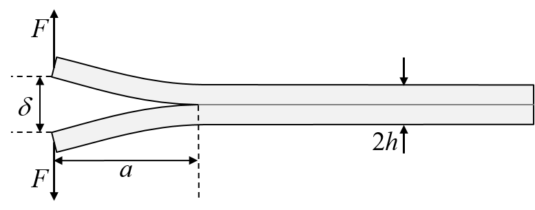
Figure-1: DCB testing
The classical way to determine the fracture energy $G_{Ic}$ in mode I require crack-length monitoring during the fracture tests, which is generally difficul to perform.
An alternative is The Compliance Based Beam Method (CBBM) using beam theory, where the fracture energy is related to the change of compliance $C$ during fracture. This is expressed by the Irwin-Kies relation:
\begin{equation} G_{Ic} = \frac{F^2}{2b}\frac{dC}{da} \tag{5} \end{equation}where the compliance is $C=\delta / F$
The compliance based on Timoshenko beam theory is:
\begin{equation} C = \frac{8 a^3}{E b h^3} + \frac{12a}{5 G b h} \tag{6} \end{equation}Combining (5) and (6) to obtain:
\begin{equation} G_{Ic} = \frac{F^2}{b^2}\ \big( \frac{12 a^2}{E h^3} + \frac{6}{5 G h} \big) \tag{7} \end{equation}Now, we solve (7) for $F$ and compute $\delta = CF$
Example:
b,h,E,G,GIc = 10, 4, 125000, 5000, 0.1

F, d = [0,], [0,]
import numpy as np
na = np.linspace(40,55,100)
tota = na[-1]-na[0] # total crack length

for a in na:
    Ft = ( (GIc*b**2)/(  ((12*a**2)/(E*h**3)) + (6/(5*G*h))  ) )**0.5
    dt = Ft*(   (8*a**3)/(E*b*h**3)  + (12*a)/(5*G*b*h)      )
    F.append(Ft)
    d.append(dt)
F.append(0)
d.append(0)

import matplotlib.pyplot as plt
%matplotlib inline
fig,ax = plt.subplots(nrows=1,ncols=1, figsize = (10,8))
ax.plot(d,F,'-',color='green')
ax.grid(True)
ax.set_xlim(0,)
ax.set_ylim(0,)
plt.show()

Verify that the area of the curves divided by the fracture area is equalt to $G_{Ic}$ using numerical integration:
energy=np.trapz(y=F,x=d)
print('GIc=',energy/(b*tota))
End-notch flexure
Intentionally left empty


