Thick laminates
The term thick laminates refers to laminates where transverse shear deformation plays a significant role. Therefore, whether a laminate is considered thick depends on multiple factors beyond just its thickness dimension.
Basic concepts
Flexural stiffness of plates and beams is proportional to the cube of the thickness, $h^3$. Hence, there is often a significant motivation for maximizing the thickness of shell-like structures. When the thickness increases relatively to lateral characteristic dimensions, the transverse shear deformation, which is neglected in classical laminate theory, becomes significant.
The shear contribution is particularly pronounced when the transverse stiffness is low compared to the in-plane stiffness. This is exceptionally true for sandwich structures having high-modulus fiber composite face sheets combined with a low density, low modulus core material. For these structures, the transverse shear deformation must be included for realistic estimations of the out-of-plane deformation.
Example
From Effective properties of laminates: the bending stiffness along the x-axis when $D_{xs}=D_{ys}=0$ is:
\begin{equation} D_b = b\big ( D_{xx} - \frac{D_{xy}^2}{D_{yy}} \big) \tag{1} \end{equation}m1= {"name": "E-glass/Epoxy", "rho": 2000E-12, "E1": 40000, "E2": 10000,
"v12": 0.3, "G12": 3800, "G13": 3800, "G23": 3400}
from laminatelib import laminateStiffnessMatrix
def bendingStiffness(layup,b=1):
# bending stiffness according to equation (1)
ADB = laminateStiffnessMatrix(layup)
return ADB[3,3] - (ADB[3,4]**2)/ADB[4,4]
When increasing the thickness by a factor two for all layers, the bending stiffness increases by a factor eight:
layup1 = [{'mat':m1, 'ori':0, 'thi': 1},
          {'mat':m1, 'ori':90, 'thi':1},
          {'mat':m1, 'ori':0, 'thi': 1} ]

layup2 = [{'mat':m1, 'ori':0, 'thi': 2},
          {'mat':m1, 'ori':90, 'thi':2},
          {'mat':m1, 'ori':0, 'thi': 2} ]

print(   bendingStiffness(layup2)/bendingStiffness(layup1)   )
The significance of transverse shear
Recall that the assumptions for the laminate theory neglect the transverse (or out-of-plane) shear stresses $\tau_{xz}$ and $\tau_{yz}$ as well as the shear strains $\gamma_{xz}$ and $\gamma_{yz}$.
For simplicity, we shall limit the initial discussion to beams with homogenous cross sections.
Consider 3-point bending of a beam with a rectangular cross section:
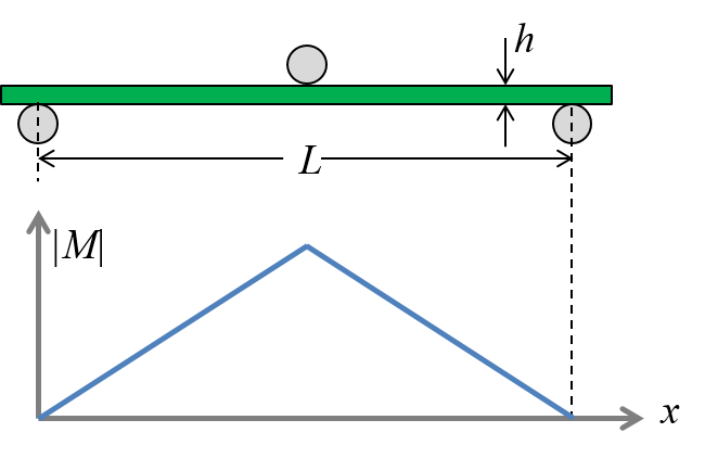
Figure-1: 3-point bending
The deflection of a freely supported beam subjected to 3-point bending according to the Euler-Bernoulli beam theory (based on the Kirchhoff assumptions, also being the basis for the laminate theory):
\begin{equation} w_{Kir} = \frac{FL^3}{48 E I} \tag{2} \end{equation}Timoshenko beam theory considers shear deformation as well:
\begin{equation} w_{Tim} = \frac{FL^3}{48 E I} + \frac{FL}{4 \kappa G b h} \tag{3} \end{equation}The ratio between the solutions of the two different assumptions is:
\begin{equation} \frac{w_{Tim}}{w_{Kir}} =1 + \frac{Eh^2}{\kappa G L^2} \tag{4} \end{equation}where the value of the Timoshenko shear coefficient $\kappa$ is dependent on Poisson's effect, but for simplicity usually approximated to be $5/6$.
Observe that the difference between the two theories increases when the ratio of $E/G$ increases, everything else being constant.
Numerical examples:
Consider an aluminum beam where the length to thickness ratio $h/L = 0.1$:
K=5/6
E = 70000
G = E/2.6
L = 100
h = 10

print(1+(E*h**2)/(K*G*L**2))
According to the result, the Timoshenko theory predicts about 3% greater deflection than the Euler-Bernoulli theory.
Now, consider a similar beam geometry having a typical UD CRFP material where the fibers are aligned with the x-axis:
K=5/6
E = 140000
G = 5000
L = 100
h = 10

print(1+(E*h**2)/(K*G*L**2))
Due to the much greater ratio of $E_1/G_{13}$, the difference is now more than 30%.
A comparative study for a range of $h/L$ ratios is presented below:
import numpy as np
h=np.linspace(1,20)

E=70000
G=E/2.6
L=200
K=5/6

deflectionRatio1 = 1+(E*np.power(h,2))/(K*G*L**2)

E=140000
G=5000

deflectionRatio2 = 1+(E*np.power(h,2))/(K*G*L**2)

import matplotlib.pyplot as plt
%matplotlib inline
fig,ax = plt.subplots(nrows=1,ncols=1, figsize = (6,4))
ax.plot(h/L,deflectionRatio1,'-',color='blue',label='Aluminum, E/G = 2.6')
ax.plot(h/L,deflectionRatio2,'-',color='green',label='UD CFRP,  E/G = 28.0')
ax.grid(True)
ax.legend(loc='best')
ax.set_title('Timoshenko versus Kirchhoff assumptions')
ax.set_xlabel('h/L',size=12)
ax.set_ylabel('Deflection ratio',size=12)
ax.set_xlim(0,)
plt.show()

The effective transverse shear stiffness of a laminate can be approximated using a thickness-weighted average of the layer shear stiffnesses:
\begin{equation} G = \frac{1}{h}\sum_{k=1}^n G_{xz,k} \cdot t_k \tag{5} \end{equation}The procedure is straight forward for laminates containing only 0-orientation and 90-orientation of layers as demonstrated in the case study Static FEA of a layered cantilever beam


