Static FEA of a layered cantilever beam
Problem statement
How simple and computationally cheap can a layered cantilever beam be modelled when only the accurate solution for the deformation is required?
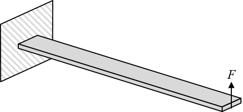
Figure-1
The layered beam for the example is subjected to two load cases:
- Flapwise loading, $F_z = 10\text{ N}$
- Edgewise loading, $F_y = 100\text{ N}$
Dimensions are: Length $L=400$ mm, width $b=25$ mm and thickness, or height, $h=5$ mm. Material and layup is given in the following code:
import matlib, laminatelib

m1=matlib.get('Carbon/Epoxy(a)')

layup = [ {'mat':m1 , 'ori': 0   , 'thi':1} ,
          {'mat':m1 , 'ori': 90  , 'thi':1} ,
          {'mat':m1 , 'ori': 0   , 'thi':1} ,
          {'mat':m1 , 'ori': 90  , 'thi':1} ,
          {'mat':m1 , 'ori': 0   , 'thi':1}  ]
Analytical solutions
Case-1: Flapwise loading
One end is fixed for all available DOF while the opposite end is subjected to the force $F_z$ in the flapwise direction.
From beam theory (see Effective properties of laminates), the flexural stiffness can be found from the components of the laminate stiffness matrix as
\begin{equation} D_f = b \big ( D_{xx} - \frac{D_{xy}^2}{D_{yy}} \big) \tag{1} \end{equation}The tip deflection included shear contribution given by Timoshenko beam theory is
\begin{equation} \delta = \frac{F_zL^3}{3D_f} + \frac{F_zL}{\kappa A G} \tag{2} \end{equation}where $G$ is taken as the average shear moduli
\begin{equation} G = \frac{1}{5}\sum_{k=1}^n G_{xz,k} \cdot t_k = \frac{1}{5}(3G_{13}+2G_{23}) \tag{3} \end{equation}L,b,h,Fz,Fy = 400,25,5,10,100
ABD = laminatelib.laminateStiffnessMatrix(layup)
Df = b*(ABD[3,3]-(ABD[3,4]**2)/ABD[4,4])
G=(3*m1['G12']+2*m1['G23'])/6
K=5/6
A=h*b
delta1 = (Fz*L**3)/(3*Df) + (Fz*L)/(K*A*G)
print('Deflection, flapwise loading = ',round(delta1,3),'mm')
Case-2: Edgewise loading
One end is fixed for all available DOF while the opposite end is subjected to the force $F_y$ in the edgewise direction.
The tip deflection included shear contribution given by Timoshenko beam theory is still
\begin{equation} \delta = \frac{FL^3}{3EI} + \frac{FL}{\kappa A G} \tag{4} \end{equation}where $E$ now is the effective modulus of the laminate given by
\begin{equation} E = \bar E_x = \frac{1}{h} \big ( A_{xx} - \frac{A_{xy}^2}{A_{yy}} \big) \tag{5} \end{equation}and
\begin{equation} I = \frac{hb^3}{12} \tag{6} \end{equation}The shear modulus $G$ is now the effective in-plane shear modulus of the laminate,
\begin{equation} G = \bar G_{xy} = \frac{1}{h} A_{ss} \tag{7} \end{equation}E=(ABD[0,0]-(ABD[0,1]**2)/ABD[1,1])/h
G=ABD[2,2]/h
K=5/6
A=5*25
I=(h*b**3)/12
delta2 = (Fy*L**3)/(3*E*I) + (Fy*L)/(K*A*G)
print('Deflection, edgewise loading = ',round(delta2,2),'mm')
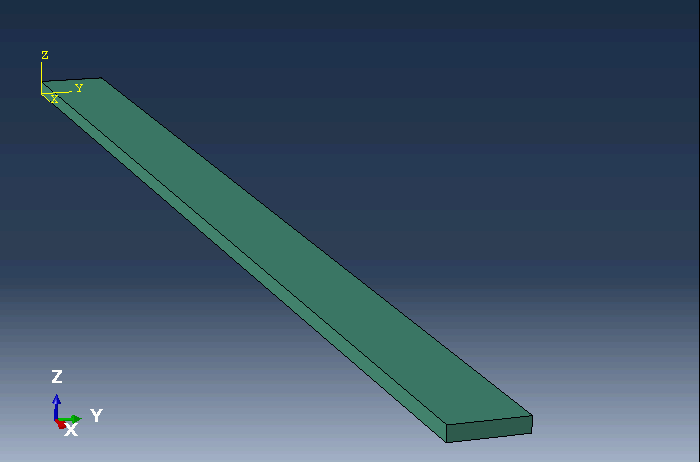
Solide models with discrete layers
The individual layers are represented by discrete cells with material orientation as specified and there must be at least one element through the thickness of individual layers. For well-shaped elements, the aspect ratio should not exceed 10. The minimum number of hex elements is therefore:
from math import ceil
n_L   = ceil( 400/10 )    # along the length
n_b   = ceil( 25/10 )     # along the width
n_t   = 5                 # through the thickness
n_tot = n_L*n_b*n_t
print(n_L, n_b, n_t, n_tot)
The model using the minimum number of C3D8R elements behaves more compliant than the corresponding model where C3D20R elements are used, the latter also being most comparable to the analytical solution. An artificially low flexural stiffness for a model having few elements of type C3D8R through the section (only 3 for edgewise mode) is as expected.

A model with C3D8R elements having two elements through the thickness of layers and element aspect ratio of 5 shows results closer to the analytical solution and to the model with C3D20R elements.
n_L   = ceil( 400/2.5 )    # along the length
n_b   = ceil( 25/2.5 )     # along the width
n_t   = 10                 # through the thickness
n_tot = n_L*n_b*n_t
print(n_L, n_b, n_t, n_tot)
| Element type | Section type | No. of elements | Flapwise, UZ | Edgewise, UY |
|---|---|---|---|---|
| (Analytical) | N/A | N/A | 7.78 | 4.06 |
| C3D8R | Discrete homogeneous | 600 | 8.03 | 4.56 |
| C3D8R | Discrete homogeneous | 16 000 | 7.84 | 4.11 |
| C3D20R | Discrete homogeneous | 600 | 7.78 | 4.07 |
| C3D20R | Discrete homogeneous | 16 000 | 7.78 | 4.07 |
Table-1: Results, solid models with discrete layers
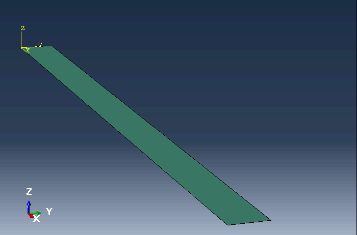
Solid models with solid composite layup
In these models the laminate is represented by a section property (layup) with only one solid element,C3D8R or C3D20R through the thickness.
Note that the layup defines thicknesses relatively to element thickness in the stack direction. Hence, if the layup contains all five layer, we can only use one element through the thickness of the beam. It is evident from the results in Table-1 that this is not an applicable solution when using the linear 8-nodes hex element with reduced integration (C3D8R) which is known to be unable to represent any reasonable bending stiffness.
| Element type | Section type | No. of elements | Flapwise, UZ | Edgewise, UY |
|---|---|---|---|---|
| (Analytical) | N/A | N/A | 7.78 | 4.06 |
| C3D8R | Composite layup | 400 | 45.80 | 4.22 |
| C3D20R | Composite layup | 8 | 8.00 | 4.05 |
| C3D20R | Composite layup | 16 | 8.02 | 4.05 |
| C3D20R | Composite layup | 64 | 8.02 | 4.06 |
| C3D20R | Composite layup | 400 | 8.02 | 4.06 |
Table-2: Results, solid models with composite layup
Shell models
The linear QUAD with reduced integration is the default choice and suitable for most problems. The S4R is a 4-node shell element with reduced integration and therefore, few elements through sections involving bending will show low bending stiffness for the structure. Observe that the example with only one element across the width produces a result that is now way near reality.
The fully integrated element S4 performs excellent for this bending problem, even with only one element across the width. This element comes however with much higher computational cost compared to S4R.
| Element type | Section type | No. of elements | Flapwise, UZ | Edgewise, UY |
|---|---|---|---|---|
| (Analytical) | N/A | N/A | 7.78 | 4.06 |
| S4R | Composite layup | 2 | 7.29 | 138 |
| S4R | Composite layup | 64 | 7.78 | 5.37 |
| S4R | Composite layup | 400 | 7.78 | 4.23 |
| S4 | Composite layup | 2 | 7.29 | 3.61 |
| S4 | Composite layup | 64 | 7.78 | 4.01 |
Table-3: Results, shell models


