FEA tool for flexural stiffness
Flexural stiffness is a critical property in mechanical engineering, as it quantifies the resistance of a structure to bending under applied loads. It plays a significant role in the design, analysis, and performance evaluation of beams and columns, plates, shells, and other structural components.
The property ensures that structural elements can support the applied bending loads or compressive forces without excessive deflection or elastic instability.
The flexural stiffness of a component also affects its natural frequencies. In dynamic systems, stiffness must be optimized to avoid resonant conditions that could lead to fatigue or failure, and properly tuned flexural stiffness can help manage energy absorption during impact.
Eventually, a proper design and optimization process for flexural stiffness enables weight minimization in lightweight design.
Flexural stiffness
Flexural stiffness $D_b$ will be define as the ratio of bending moment to the curvature $\kappa$
\begin{equation} D_b = \frac{M}{\kappa} \tag{1} \end{equation}The flexural stiffness of a simple homogeneous cross section can easily be obtained. For example, the value for a rectangular solid section is given by:
\begin{equation} D_b = EI = E \frac{bh^3}{12} \tag{2} \end{equation}The idea for this case study is to develop a finite element tool (Abaqus script) capable of computing the flexural stiffness of more complex structures, including non-constant cross sections along the length of the component.
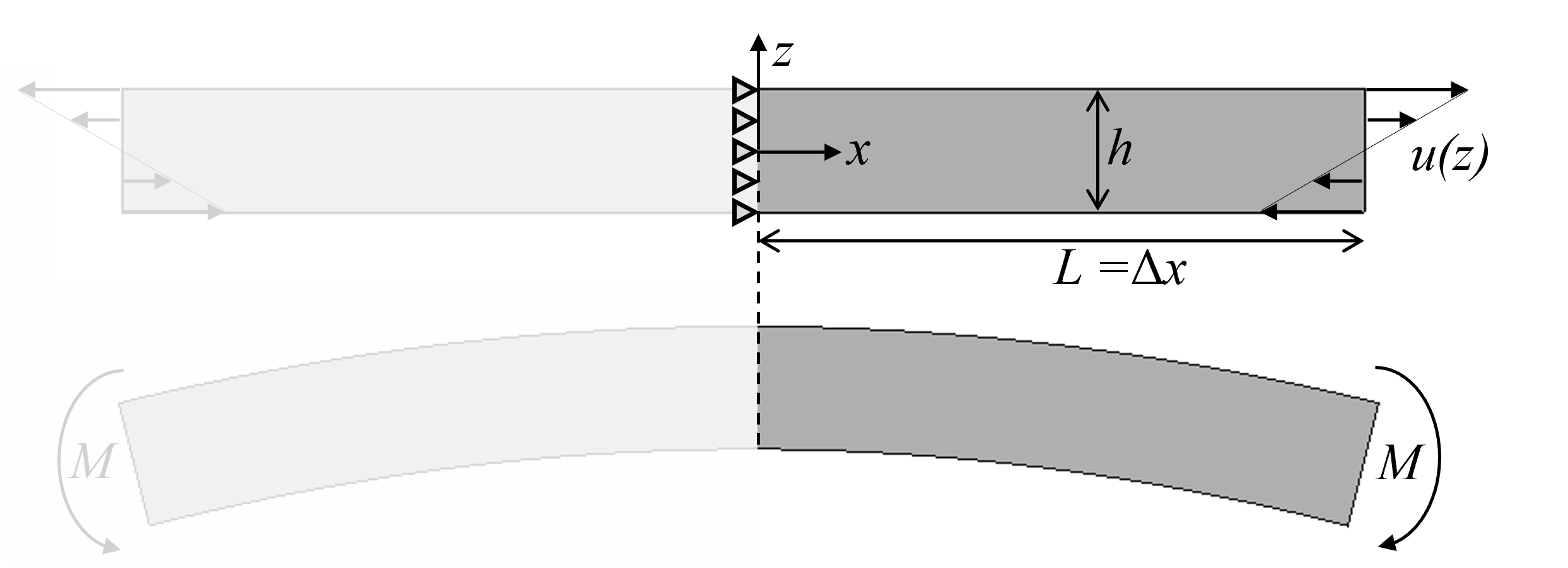
Deformation
The neutral plane is located at the midplane where $z=0$.
The nodes at minimum $x$ will be fixed in the $x$-direction:
\begin{equation} u_{min}(z) = 0 \tag{3} \end{equation}while a linear displacement field is assumed at the opposite end,
\begin{equation} u_{max}(z) = c\cdot z \tag{4} \end{equation}The strain as function of $z$ is therefore
\begin{equation} \varepsilon_x = \frac{du}{dx} = \frac{\Delta u(z)}{L} = \frac{c\cdot z}{L} \tag{5} \end{equation}The relation between strain and curvature along $x$ is
\begin{equation} \varepsilon_x = \kappa_x z \tag{6} \end{equation}such that
\begin{equation} \frac{c\cdot z}{L} = \kappa_x z \Rightarrow c = \kappa_x L \tag{7} \end{equation}Moment
The moment can be found from the sum of the nodal reaction forces $f_i$ in the $x$-direction multiplied by the corresponding z-coordinates $z_i$:
\begin{equation} M = \sum f_i \cdot z_i \tag{8} \end{equation}and the flexural stiffness is finally computed by equation (1).
FEA Implementation
A simple brick will be used for testing and benchmarking:
from abaqus import *
from abaqusConstants import *

def demoBrick(modelname, X, Y, Z, esize, E, nu):
    mod = mdb.Model(name=modelname, modelType=STANDARD_EXPLICIT)
    ske = mod.ConstrainedSketch(name='__profile__', sheetSize=200.0)
    ske.rectangle(point1=(0.0, 0.0), point2=(X, Y))
    prt = mod.Part(name='Brick', dimensionality=THREE_D, type=DEFORMABLE_BODY)
    prt.BaseSolidExtrude(sketch=ske, depth=Z)
    del ske
    mat = mod.Material(name='Material-1')
    mat.Elastic(table=((E, nu), ))
    mod.HomogeneousSolidSection(name='Section-1', material='Material-1', thickness=None)
    region = prt.Set(cells=prt.cells, name='Set-1')
    prt.SectionAssignment(region=region, sectionName='Section-1')
    import mesh
    elemType1 = mesh.ElemType(elemCode=C3D20R, elemLibrary=STANDARD)
    regions =(prt.cells, )
    prt.setElementType(regions=regions, elemTypes=(elemType1,))
    prt.seedPart(size=esize, deviationFactor=0.1, minSizeFactor=0.1)
    prt.generateMesh()
    ass = mod.rootAssembly
    ass.DatumCsysByDefault(CARTESIAN)
    ass.Instance(name='Bricki', part=prt, dependent=ON)

modelname = 'Demo1'
demoBrick(modelname=modelname, X = 20, Y = 20, Z = 5, esize = 2, E = 100000.0, nu = 0.3)
The idea is to create a code that takes any representative model that has been prepared within the following limitations:
- The assembly of the model has only one solid element instance
- The instance has section and material assignments
- The instance has a mesh
- The bending stiffness will be computed along the x-direction and about the y-axis
- Periodicity is or symmettry conditions are assumed in the x-direction
The code will be implemented as a function that takes a minimum of parameters: the model name modelname, a geometric tolerance tol and the imposed kurvature K. The tolerance will serve as a flexible way to select nodes of any models that are not precise:
def solveFlexStiff(modelname,tol,K):
    from mesh import MeshNodeArray       # in order to convert from a list of nodes to a MeshNodeArray
    mod = mdb.models[modelname]          # pointer to the model
    ass = mod.rootAssembly               # pointer to the assembly
    insname = ass.instances.keys()[0]    # Assuming there is only one instance (therefore the first, [0])
    ins = ass.instances[insname]         # pointer to the single instance
Geometrical parameters
Dimensions are not supposed to be provided in the script, but needs to be found. A simple addition finds the dimensions based on nodes:
    dims = ins.nodes.getBoundingBox()
    xmin, ymin, zmin = dims['low']
    xmax, ymax, zmax = dims['high']
    dx, dy, dz = xmax-xmin, ymax-ymin, zmax-zmin
The height h and width b are directly connected to the dimensions, while the z-coordinate z0 to the mid-plane must be computed:
h, b, z0 = dz, dy, (zmin+zmax)/2.0Selecting and creating sets
Nodes at minimum minimum x as well as maximum shall be subjected to displacements according to (3) and (4). Hence, they must be found and put into sets:
    nodes_minX = ins.nodes.getByBoundingBox(xMin=xmin-tol,xMax=xmin+tol)
    nodes_maxX = ins.nodes.getByBoundingBox(xMin=xmax-tol,xMax=xmax+tol)
    region_minX = ass.Set(nodes = nodes_minX, name='nodes-minX')
    region_maxX = ass.Set(nodes = nodes_maxX, name='nodes-maxX')
Two nodes are required for for preventing rigid body motion. An easy way out could be to select one node as the corner at xmin, ymin, zmin and the other at xmin, ymax, zmin. However, there could easilly be models of profiles where these are empty positions. Hence, a different strategy is needed. The following approach should be relatively robust for any profiles as long as there are more than one node at the minimum value of z on the face at minimum x:
    tempdims = nodes_minX.getBoundingBox()
    tempxmin, tempymin, tempzmin = tempdims['low']
    tempnodes = nodes_minX.getByBoundingBox(zMin=tempxmin-tol, zMax=tempxmin+tol)
    tempdims = tempnodes.getBoundingBox()
    tempxmin, tempymin, tempzmin = tempdims['low']
    tempxmax, tempymax, tempzmax = tempdims['high']
    nodeRB1 = ins.nodes.getByBoundingSphere(center = (tempxmin, tempymin, tempzmin), radius=tol)
    nodeRB2 = ins.nodes.getByBoundingSphere(center = (tempxmin, tempymax, tempzmin), radius=tol)
    if len(nodeRB1) != 1 or len(nodeRB2) !=1:
        print 'Something wrong'
        return
    regionRB1 = ass.Set(nodes = nodeRB1, name='node-rb1')
    regionRB2 = ass.Set(nodes = nodeRB2, name='node-rb2')
Step and boundary conditions
Creating a static step
mod.StaticStep(name='Step-1', previous='Initial')And boundary condition according to (3):
mod.DisplacementBC(name='U1-XMIN', createStepName='Step-1', region=region_minX, u1=0.0)An analytic field will be used to impose the displacement $u$ on the surface at maximum x-coordinates:
    mod.ExpressionField(name='AnalyticalField-1', expression=' ( Z -{})*{}'.format(z0,dx*K))
    mod.DisplacementBC(name='U1-L2', createStepName='Step-1', region=region_maxX, u1=1.0,
        amplitude=UNSET, fixed=OFF, distributionType=FIELD, fieldName='AnalyticalField-1', localCsys=None)
Example: zmim is 0 while zmax is 5.
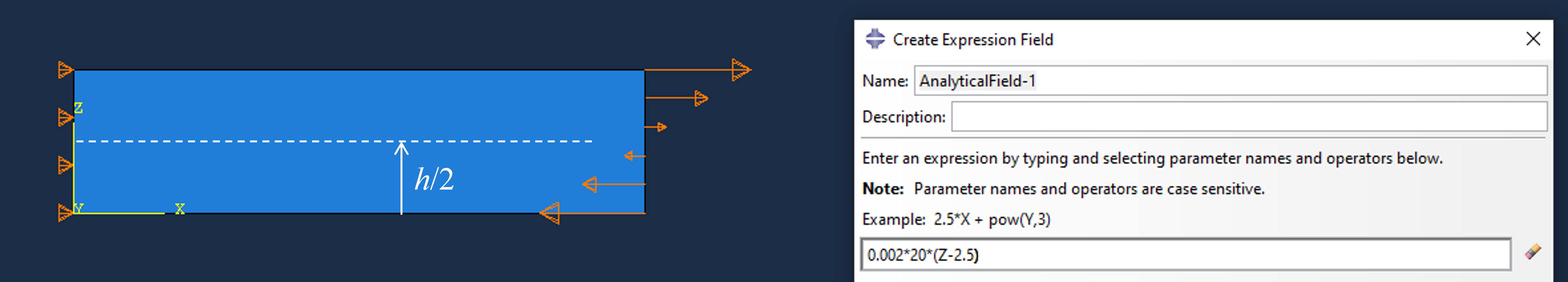
Let $X,Y,Z$ be the axes or coordinates of the global coordinate system, while the local coordinates of the brick is $x,y,z$. The midplane of the brick is displaced by $h/2$ such that the analytical field becomes
$$u = \kappa_x L \cdot z = \kappa_x L(Z-h/2)$$Hence, with the parameters $L=20, \kappa_x = 0.002, h=5$, the expression must be 0.002*20*(Z-2.5) for the current example.
Preventing rigid body motion:
    mod.DisplacementBC(name='RB1', createStepName='Step-1', region=regionRB1, u2=0.0, u3=0.0)
    mod.DisplacementBC(name='RB2', createStepName='Step-1', region=regionRB2, u3=0.0)
Job and results
    job = mdb.Job(name=modelname, model=modelname)
    job.submit(consistencyChecking=OFF)
    job.waitForCompletion()
    odb = session.openOdb(name=modelname + '.odb')
    odb_regionL2=odb.rootAssembly.nodeSets['NODES-MAXX']
    fieldRF_regionL2 = odb.steps['Step-1'].frames[-1].fieldOutputs['RF'].getSubset(region = odb_regionL2)
    Mi = []
    for node, value in zip(region_maxX.nodes, fieldRF_regionL2.values):
        z = node.coordinates[2]-z0
        fx = value.data[0]
        Mi.append(fx*z)
    M = sum(Mi)
    EI_fea = M/K
    print 'EI_fea = {}'.format(EI_fea)
Example 1
modelname = 'Demo1'
demoBrick(modelname=modelname, X = 20, Y = 20, Z = 5, esize = 2, E = 100000.0, nu = 0.3)
solveFlexStiff(modelname=modelname, tol=0.1, K=0.002)
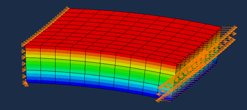
Result print out: EI_fea = 20833338.4526
Analytic solution:
E, b, h = 100000, 20, 5
EI = E*(b*h**3)/12
print('EI={}'.format(EI))
Example 2
An aluminum profile, manually modeled:
solveFlexStiff(modelname='Demo2', tol=0.1, K=0.002)
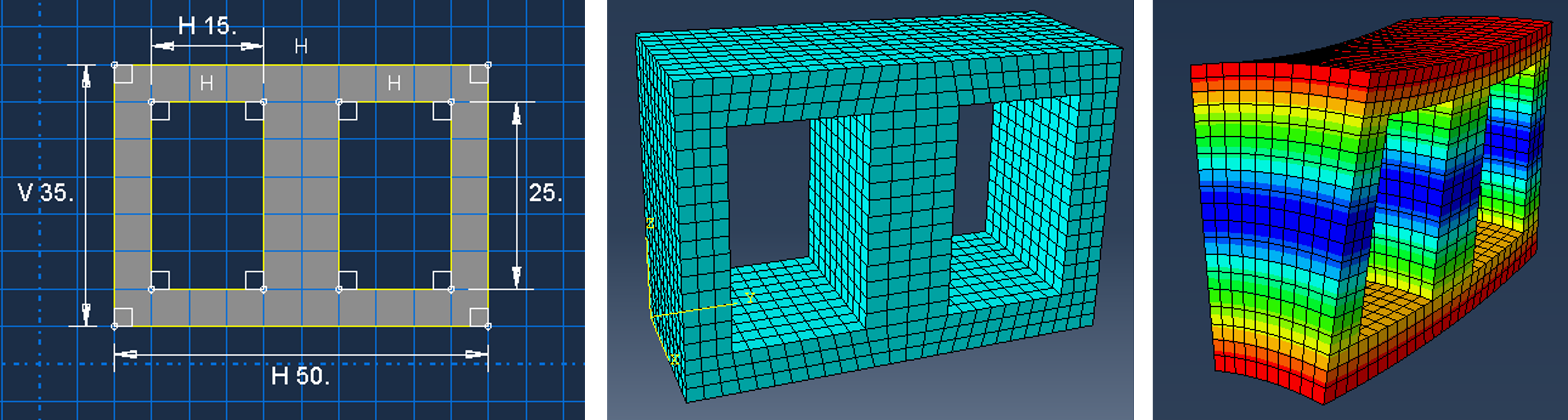
Result: EI_fea = 9752170308.51
Analytic solution:
E = 70000
EI = E*((50*35**3)/12 - (30*25**3)/12)
print('EI={}'.format(EI))
Complete script
from abaqus import *
from abaqusConstants import *

def demoBrick(modelname, X, Y, Z, esize, E, nu):
    mod = mdb.Model(name=modelname, modelType=STANDARD_EXPLICIT)
    ske = mod.ConstrainedSketch(name='__profile__', sheetSize=200.0)
    ske.rectangle(point1=(0.0, 0.0), point2=(X, Y))
    prt = mod.Part(name='Brick', dimensionality=THREE_D, type=DEFORMABLE_BODY)
    prt.BaseSolidExtrude(sketch=ske, depth=Z)
    del ske
    mat = mod.Material(name='Material-1')
    mat.Elastic(table=((E, nu), ))
    mod.HomogeneousSolidSection(name='Section-1', material='Material-1', thickness=None)
    region = prt.Set(cells=prt.cells, name='Set-1')
    prt.SectionAssignment(region=region, sectionName='Section-1')
    import mesh
    elemType1 = mesh.ElemType(elemCode=C3D20R, elemLibrary=STANDARD)
    regions =(prt.cells, )
    prt.setElementType(regions=regions, elemTypes=(elemType1,))
    prt.seedPart(size=esize, deviationFactor=0.1, minSizeFactor=0.1)
    prt.generateMesh()
    ass = mod.rootAssembly
    ass.DatumCsysByDefault(CARTESIAN)
    ass.Instance(name='Bricki', part=prt, dependent=ON)


def solveFlexStiff(modelname,tol,K):
    from mesh import MeshNodeArray       # in order to convert from a list of nodes to a MeshNodeArray
    mod = mdb.models[modelname]          # pointer to the model
    ass = mod.rootAssembly               # pointer to the assembly
    insname = ass.instances.keys()[0]    # Assuming there is only one instance (therefore the first, [0])
    ins = ass.instances[insname]         # pointer to the single instance

    # Finding the extreem coordinates based on nodes:
    dims = ins.nodes.getBoundingBox()
    xmin, ymin, zmin = dims['low']
    xmax, ymax, zmax = dims['high']

    # Dimensions and geometrical parameters:
    dx, dy, dz = xmax-xmin, ymax-ymin, zmax-zmin
    h, b, z0 = dz, dy, (zmin+zmax)/2.0

    # Sets and regions
    nodes_minX = ins.nodes.getByBoundingBox(xMin=xmin-tol,xMax=xmin+tol)
    nodes_maxX = ins.nodes.getByBoundingBox(xMin=xmax-tol,xMax=xmax+tol)
    region_minX = ass.Set(nodes = nodes_minX, name='nodes-minX')
    region_maxX = ass.Set(nodes = nodes_maxX, name='nodes-maxX')
    tempdims = nodes_minX.getBoundingBox()
    tempxmin, tempymin, tempzmin = tempdims['low']
    tempnodes = nodes_minX.getByBoundingBox(zMin=tempxmin-tol, zMax=tempxmin+tol)
    tempdims = tempnodes.getBoundingBox()
    tempxmin, tempymin, tempzmin = tempdims['low']
    tempxmax, tempymax, tempzmax = tempdims['high']
    nodeRB1 = ins.nodes.getByBoundingSphere(center = (tempxmin, tempymin, tempzmin), radius=tol)
    nodeRB2 = ins.nodes.getByBoundingSphere(center = (tempxmin, tempymax, tempzmin), radius=tol)
    if len(nodeRB1) != 1 or len(nodeRB2) !=1:
        print 'Something wrong'
        return
    regionRB1 = ass.Set(nodes = nodeRB1, name='node-rb1')
    regionRB2 = ass.Set(nodes = nodeRB2, name='node-rb2')

    # Step and boundary conditions:
    mod.StaticStep(name='Step-1', previous='Initial')
    mod.DisplacementBC(name='U1-XMIN', createStepName='Step-1', region=region_minX, u1=0.0)
    mod.ExpressionField(name='AnalyticalField-1', expression=' ( Z -{})*{}'.format(z0,dx*K))
    mod.DisplacementBC(name='U1-L2', createStepName='Step-1', region=region_maxX, u1=1.0,
        amplitude=UNSET, fixed=OFF, distributionType=FIELD, fieldName='AnalyticalField-1', localCsys=None)
    mod.DisplacementBC(name='RB1', createStepName='Step-1', region=regionRB1, u2=0.0, u3=0.0)
    mod.DisplacementBC(name='RB2', createStepName='Step-1', region=regionRB2, u3=0.0)

    # Job and results
    job = mdb.Job(name=modelname, model=modelname)
    job.submit(consistencyChecking=OFF)
    job.waitForCompletion()
    odb = session.openOdb(name=modelname + '.odb')
    odb_regionL2=odb.rootAssembly.nodeSets['NODES-MAXX']
    fieldRF_regionL2 = odb.steps['Step-1'].frames[-1].fieldOutputs['RF'].getSubset(region = odb_regionL2)
    Mi = []
    for node, value in zip(region_maxX.nodes, fieldRF_regionL2.values):
        z = node.coordinates[2]-z0
        fx = value.data[0]
        Mi.append(fx*z)
    M = sum(Mi)
    EI_fea = M/K
    print 'EI_fea = {}'.format(EI_fea)

modelname = 'Demo1'
demoBrick(modelname=modelname, X = 20, Y = 20, Z = 5, esize = 2, E = 100000.0, nu = 0.3)
solveFlexStiff(modelname=modelname, tol=0.1, K=0.002)
Cylindrical bending
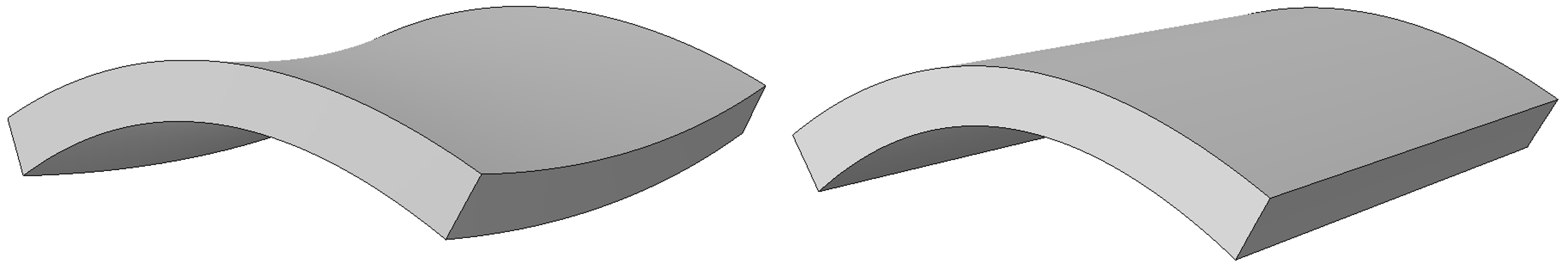
Panels, where the width is large compared to the thickness, tends to conform towards cylindrical bending as illustrated to the right. This is particularily true with the boundary conditions and loading that apply in the 3-point bending configuration explored in the case study Lightweight panel. In effect, the curvature in the transverse direction will be constrained by both the boundary conditions (supports and line load) as well as the geometrical shape that emerges during loading. The panel will therefore exhibit stiffer behavior.
The effect is directly connected to the Poisson's effect, where the modulus $E$ in (2) can be modified to the longitudinal stiffness experienced when the transverse strain is constrained ( $\varepsilon_y = 0$). That is:
$$ \varepsilon_x = \frac{1}{E} \sigma_x - \frac{\nu}{E}\sigma_y \\ \varepsilon_x = -\frac{\nu}{E} \sigma_x + \frac{1}{E} \sigma_y $$Solving for stresses when $\varepsilon_y = 0$:
\begin{equation} \sigma_x = \frac{E}{1-\nu^2} \varepsilon_x \tag{9} \end{equation}Hence, equation (2) when assuming cylindrical bending of a panel with rectangular solid homogeneous cross section takes the form
\begin{equation} D_b = \frac{E}{1-\nu^2} \frac{bh^3}{12} \tag{10} \end{equation}FEA implementation (addition)


