Composite drive shaft
Assumptions: the drive shaft can be approximated to a thin-walled tube where edge effects are neglected, see the case studies Lightweight drive shaft and Thin-walled pipes.
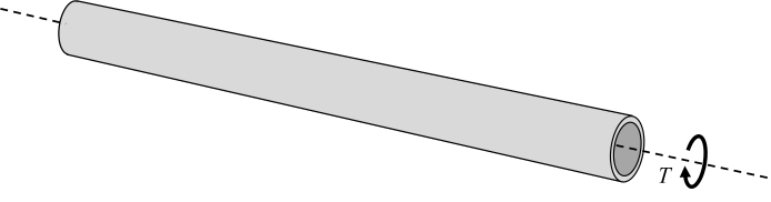
The relation between the shear section force $N_{xy}$ and the torque $T$ is now
\begin{equation} N_{xy}=\frac{T}{2\pi R^2} \tag{1} \end{equation}Hence, the governing set of equations is:
\begin{equation} \begin{bmatrix} 0 \\ 0 \\ N_{xy} \end{bmatrix} = \begin{bmatrix} A_{xx} & A_{xy} & A_{xs} \\ A_{xy} & A_{yy} & A_{ys} \\ A_{xs} & A_{ys} & A_{ss} \end{bmatrix} \begin{bmatrix} \varepsilon_x^0 \\ \varepsilon_y^0 \\ \gamma_{xy}^0 \end{bmatrix} \tag{2} \end{equation}For a balanced laminate, the only non-trivial equation is:
\begin{equation} N_{xy}=A_{ss}\gamma_{xy}^0 \tag{3} \end{equation}Solution for a homogenous isotropic drive shaft
From equation (1),
\begin{equation} \tau_{xy}=\frac{T}{2\pi R^2 t} \tag{4} \end{equation}The von Mises stress is now
\begin{equation} \sigma_{v}=\sqrt{3}\tau_{xy} \tag{5} \end{equation}Consider the following requirements and parameters for a steel shaft:
- Design torque: 5 kNm,
- Yield strength: 750 MPa (quite high yield strength)
- Fixed outer radius: 30 mm
- Wall thicness is a free parameter
Computing the required thickness and resulting mass per length:
In [1]:
from math import pi
import numpy as np

T=5E6 #Nmm
E,v,rho = 200000, 0.3, 7800E-12
G=E/(2+2*v)
Ro=30

def misesAndMass(t):
    Ri=Ro-t
    R=(Ro+Ri)/2
    tau=T/(2*pi*t*R**2)
    mises=(3**0.5)*tau
    mass=rho*pi*(Ro**2 - Ri**2)*1E6
    return (mises,mass)


thi = np.linspace(2,3,10000)
for t in thi:
    mises,mass_steel=misesAndMass(t)
    if mises<750:
        break

print('Thickness=   ',round(t,3),'mm')
print('Mises stress=',round(mises,1),'MPa')
print('Mass=        ', round(mass_steel,3),'kg/m')
A carbon fiber composite solution:
In [2]:
import laminatelib
import matlib
import numpy as np
from numpy import pi
import matplotlib.pyplot as plt
m1=matlib.get('Carbon/Epoxy(a)')

def driveShaftStuff(angle,t,R,T):
    layup =[{'mat':m1, 'ori':-angle, 'thi':t/2},
            {'mat':m1, 'ori':+angle, 'thi':t/2}]
    Ass=laminatelib.laminateStiffnessMatrix(layup)[5,5]
    Nxy=T/(2*pi*R**2)
    gxy0 = Nxy/Ass
    deformations=np.array([0,0,gxy0,0,0,0])
    res = laminatelib.layerResults(layup,deformations)
    return res[0]['fail']

angles=np.linspace(30,60)
fE_MS = [driveShaftStuff(angle,t=1, R=30,T=5E6)['MS']['bot'] for angle in angles]
plt.plot(angles,fE_MS)
plt.show()

The optimum angle is clearly 45 degrees.
In [3]:
Ro=30
t=3.5
Ri=Ro-t
R=(Ro+Ri)/2
driveShaftStuff(45,t=t, R=R,T=5E6)
Out[3]:
In [4]:
mass_cfrp=m1['rho']*pi*(Ro**2 - Ri**2)*1E6
print('Mass pr. meter', mass_cfrp,'kg')
In [5]:
mass_cfrp/mass_steel
Out[5]:


