Lightweight drive shaft
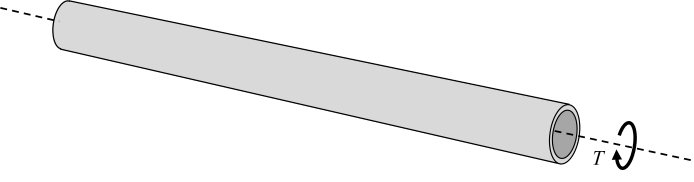
The primary function of a drive shaft is to transmit torque and rotation from one part of a machine to another.
Stage-1: Simplified stress based assessment
A thin-walled tube refers to a cylindrical structure where the wall thickness is small compared to its diameter. In engineering and mechanics, a tube is considered thin-walled if the ratio of its wall thickness to its outer diameter is less than about 1/10.
Assuming that the drive shaft resembles a thin-walled tube, the shear force caused by a torque $T$ in a cross section far from the edges is
\begin{equation} F_s = \frac{T}{r} \tag{1} \end{equation}The shear stress in a homogeneous cross section is therefore
\begin{equation} \tau=\frac{T}{2\pi r^2 t} \tag{2} \end{equation}The required wall thickness for a fixed radius, torque and allowable shear stress is therefore
\begin{equation} t=\frac{T}{2\pi r^2 \tau} \tag{3} \end{equation}The mass of the solution is the volume of the material multiplied with the density of the material:
$$m = V \rho = 2 \pi r t L \rho \Rightarrow$$\begin{equation} m = \frac{T L}{r \tau} \rho \tag{4} \end{equation}Hence, if the radius is the only free variable, the mass will be inversely proportional to the radius,
\begin{equation} m = c_1 \frac{1}{r}, \quad c_1 = \text{constant} \tag{5} \end{equation}which suggests that the radius should be maximized for a minimum weight solution:
$$ \min{(m)} \Rightarrow \max{(r)}$$Generally, the radius cannot be infinite but rather limited by constraints in the design space.
Numerical example
Data and constraints:
- Length: 1 m
- Torque: 1000 Nm
- Maximum radius according to the design space: 50 mm
- Material: steel
- Yield strength: 400 MPa
- The von Mises stress must not exceed the yield strength
The von Mises stress for a pure shear stress is
$$\sigma_{v}=\sqrt{3}\tau$$which implies that
$$\sigma_{yield} \ge \sqrt{3}\tau \Rightarrow$$\begin{equation} \tau \le \frac{\sigma_{yield}}{\sqrt{3}} \tag{6} \end{equation}import numpy as np
import matplotlib.pyplot as plt
L = 1000 # Length [mm]
T = 1E6 # Torque [N mm] (= 1000 [N m])
rho = 7850E-12 # Density, steel [Mg/mm3] (=7850 [kg/m3])
sy = 400 # Yield strength [MPa]
r = np.linspace(25, 50, 11) # radi to compute [mm]
tau = sy/(3**(1/2)) # Allowable shear stress
t = (T)/(2*np.pi*r**2*tau) # Computed thickness [mm]
m = (T*L*rho)/(r*tau) # Computed mass [Mg]
plt.plot(r,m*1E3, label='Mass [kg]')
plt.plot(r,t, label='Thickness [mm]')
plt.xlim(25,50)
plt.ylim(0,)
plt.xlabel('Radius [mm]')
plt.ylabel('Mass [kg] and Thickness [mm]')
plt.grid()
plt.legend()
plt.show()
print(' r[mm] t[mm] m[kg]')
for ri, ti, mi in zip(r,t,m):
print('{:6.1f} {:4.2f} {:4.2f}'.format(ri,ti, mi*1000))

Stage-2: Torsional buckling
The results from the previous stage suggest that the radius should be maximized for a lightweight solution. The thickness can, however, not be infinitely thin. At some point, the governing failure will be caused by elastic instability (buckling) rather than material shear failure as the thickness is reduced.
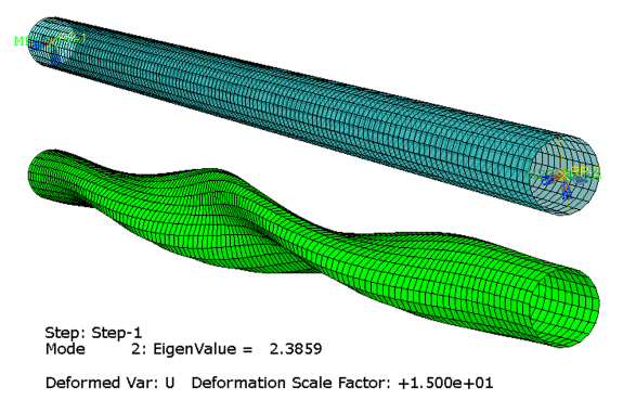
Analytical solutions for torsional buckling is rather involved and out of scope in this course. The problem can however easily be solved by a simple FEA model as presented in Abaqus Scripting, Example: Drive shaft
The model is shell based, as one simple cylinder, and the solution is a Linear perturbation - Buckling. It is assumed that both ends are connected to infinitely stiff components, simplified as MPC (multipoint constraints) where a reference point controls the displacement of all nodes on one end.
The drive shaft is subjected to a torque equal to 1000 Nm = 1E6 Nmm, and the result includes the deformed shape and the eigenvalue that shall be interpreted as a load proportionality factor (LPF). For instance, the eigenvalue for the driveshaft having a radius equal to 25 mm is 2.3859 for the applied element size shown, implying that the critical buckling load is that value multiplied with the applied torque. Thus, the eigenvalue must be greater than 1.0 for the drive shaft not to fail.
From the previous stage, the required thicknesses for corresponding radii are
print([round(ti,4) for ti in t])
print([ri for ri in r])
Using theese values in the buckling simulation, results in the following realation between radius, thickness and eigenvalue:

According to the results, solutions that are weight optimized with respect to the yield strength, will fail due to buckling when the radius is greater than about 32 mm (when the eigenvalue is greater than 1.0). Consequently, the optimal solution so far is the one where radius is approximatly 32 mm and the corresponding required thickness is about 0.70 mm. For these dimensions, the weight is slightly less than 1.1 kg.
Concluding remarks
The study examplifies that design space should generally be explored (in this case, radi in the allowable range). Furthermore, the optimum solution must typically take several issues into consideration simultaneously, such as both material strength and buckling.
There are however many important aspects missing in this study:
Safety factors: Optimization with safety factors included, may fundamentally alter the situation and consequently the resulting solution.
Materials selection: The study did not explore anything but a steel with specific properties. Alternative materials could for example be aluminum alloys which would allow for greater wall thickness for any given mass. As a consequence, torsional buckling would then become less critical and the resulting design will more likely be governed by the material strength rather than elastic instability.
Joints: The interconnection between the tube and the end joints is not trivial and will be very dependent on the selection of materials. For example, the joining av dissimilar materials has different options than the joining of similar materials. Consequently, the weight of the joints will be very influenced by the solution for the cylindrical part.


