FEA of a sandwich beam
FEA based on shell models and analytical solutions can efficiently solve for deformation, section forces, moments and stresses far from boundary conditions and sharp loads on a sandwich structure. Shell models and the simple analytical solutions are however unable to capture local effects as will be demonstrated in this study.
The object for the study is a sandwich beam, freely supported and subjected to a central line load as illustrated in Figure-1. The length between the supports are $L$ = 250 mm, and the width is $b$ = 30 mm. The beam extends additionally 10 mm at both ends.
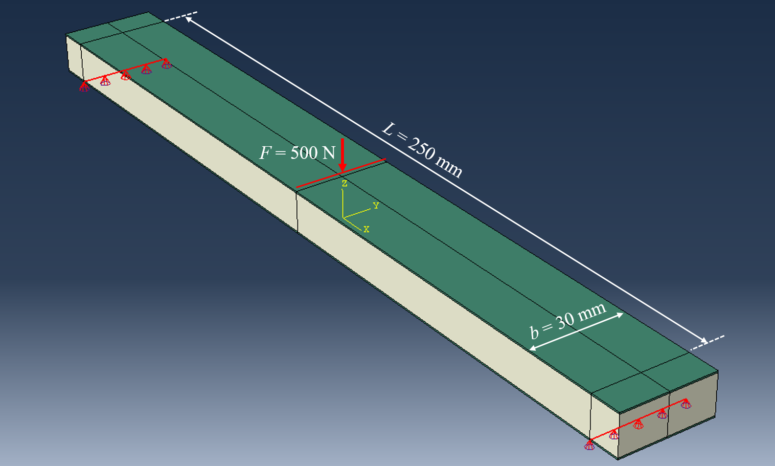
Figure-1: Dimensions
The core material and the face-sheet material have the following properties:
# Properties of core material and homogenized face sheet material:

mcore={'name':'H100','rho':100E-12, 'E1':100, 'E2':100,
       'E1':100, 'E2':100, 'E2':100,
       'v12':0.3, 'v12':0.3, 'v12':0.3,
       'G12': 38.5, 'G13': 38.5, 'G23': 38.5 }

mcfrp={'name':'Woven Carbon/epoxy','rho':1580E-12,
       'E1': 59000, 'E2': 59000, 'E3': 9200,
       'v12': 0.045, 'v13' :0.462, 'v23': 0.462,
       'G12': 2750, 'G13': 2700, 'G23': 2700 }
The core material, a cross-linked PVC foam, is assumed to be isotropic, while the face-sheet material is a homogenized laminate of woven carbon fiber and epoxy.
The thickness of the core is $h_c$ = 12 mm and each face-sheets has a thickness $t_f$ = 0.5 mm as illustrated in Figure-2. In order to obtain high fidelity, a very fine mesh of C3D20R elements is used, and there are two elements through the thickness of both face-sheets.
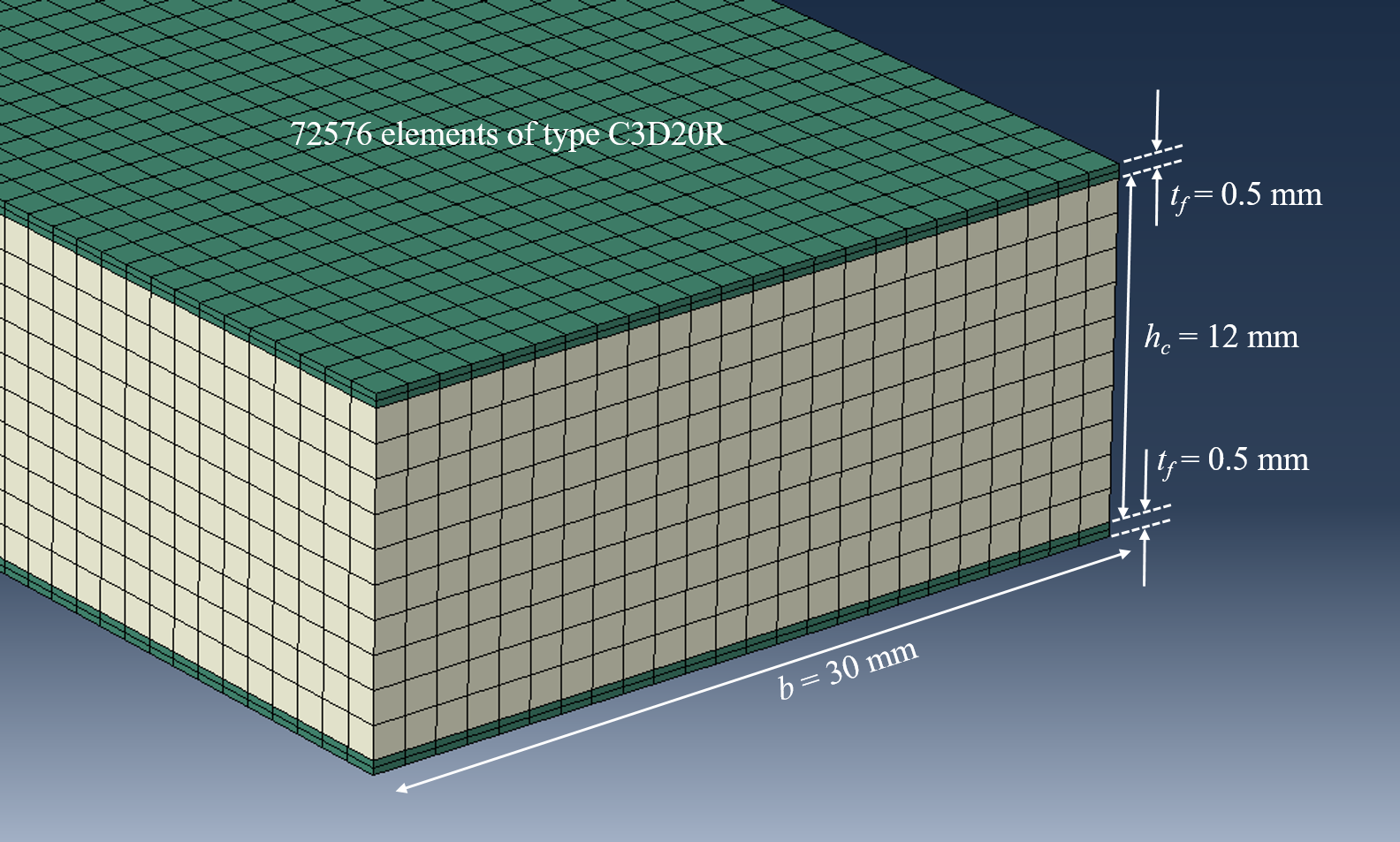
Figure-2: Dimensions and mesh
The boundary condition for the support and the centerline load is illustrated in Figure-1. Note that there must be additional boundary conditions to prevent rigid body motions.
The approach for the center load consist of a coupling for the uz degree of freedom between the center point and all nodes along the centerline. This approach resembles a rigid, sharp member imposing a line load on the top-face of the sandwich.
The problem involves relatively small deformation, and a small deformation static solution is therefore chosen.
Analytical solution
From simplified approximations for sandwich:
The maximum deflection is a superposition of bending and shear deformation
\begin{equation} \delta = \frac{FL^3}{48D_b} + \frac{FL}{4S} \tag{1} \end{equation}where
\begin{equation} D_b = \frac{E_f t_f b h^2}{2}, \quad S = b h G_c, \quad \text{and} \quad h = h_c + t_f, \tag{2} \end{equation}Max/min stress is:
\begin{equation} \sigma = \pm \frac{FL}{4 b h t_f} \tag{3} \end{equation}L,b,F,hc,tf = 250, 30, 500, 12, 0.5
h = hc + tf
Ef = mcfrp['E1']
Gc = mcore['G13']
Db = (Ef*tf*b*h**2)/2
S = b*h*Gc
delta = (F*L**3)/(48*Db) + (F*L)/(4*S)
print('Deflection = ',round(delta,3),'mm')
sigma=(F*L)/(4*b*h*tf)
print('Maxium stress =',round(sigma,3), 'MPa')
Solid model results
As evident from Figure-3, the compressive longitudinal stress on top face along the line load exceeds the analytical value by a factor 509/167 ≈ 3. The tensile stress is from the FEA model is also significant greater than the result from the analytical solution (204/167 ≈ 1.2)
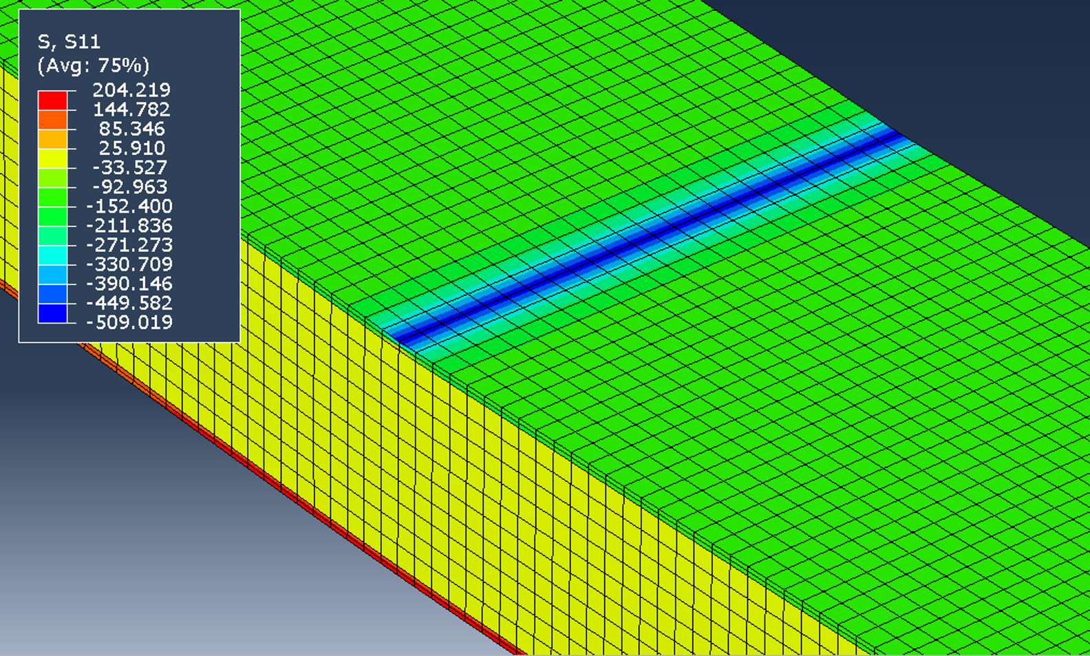
Figure-3: Longitudinal stress
The compressive through-the-thickness strain shown in Figure-4 is not available from a shell model or from a simple analytical model. Because of this compressive strain, the deflection measured at the top face will be slightly different from the deflection measured at the bottom face as illustrated in Figure-5. Note however that the analytical solution (-4.519 mm) is in well agreement with the FEA solution (-4.505) measured at the top face.
The transverse shear strain is clearly shown in Figure-6 where a deformation-scaling factor of 10 has been used.
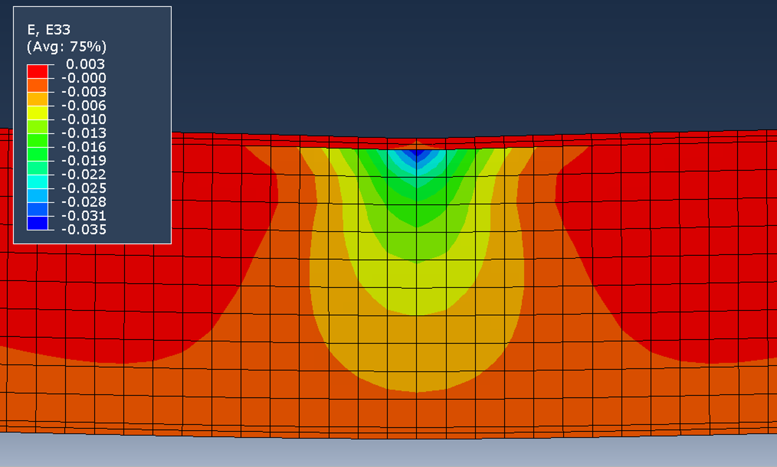
Figure-4: Through-the-thickness strain
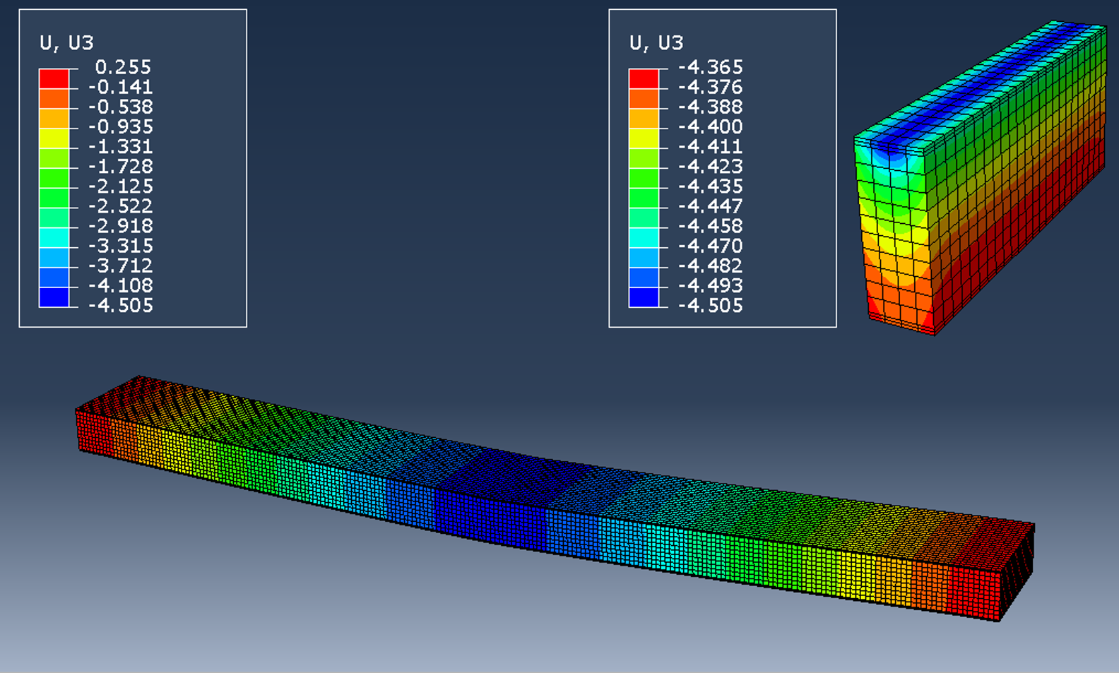
Figure-5: Deflection measured by displacement in the z-direction
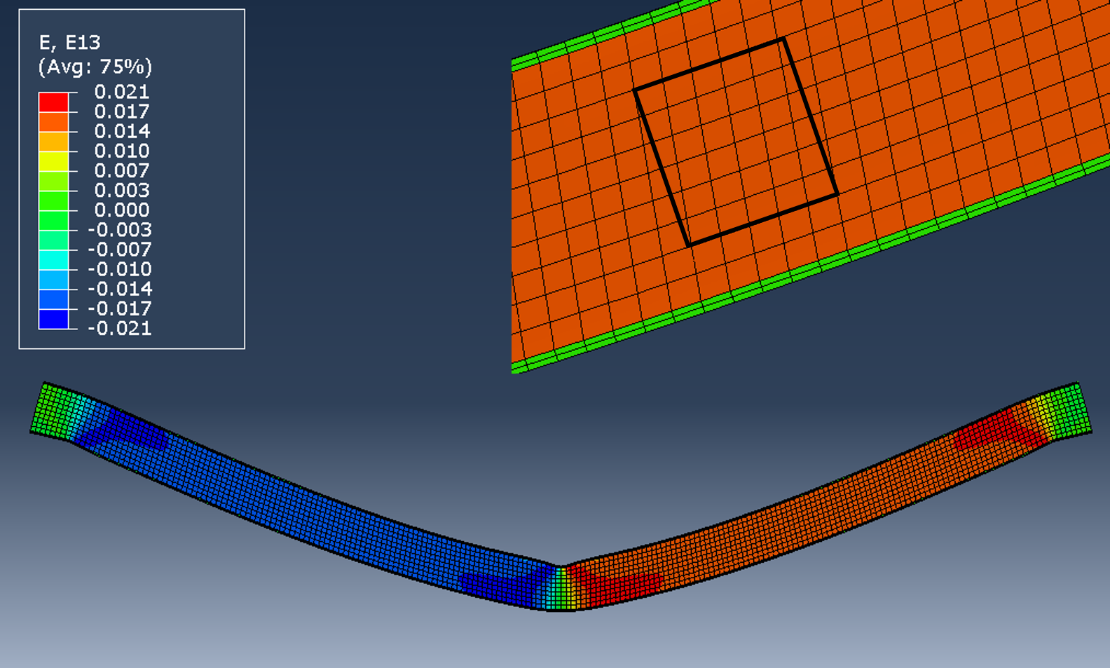
Figure-6: Shear deformation (scale factor = 10) and transverse shear strain
The longitudinal stress along an edge from one end to the other is extracted at both the top face and the bottom face. The results are shown in Figure-7 and Figure-8 along with the analytical solutions. Note that the stress from the analytical solution is proportional to the bending moment, thus varying linearly from the support to the center of the beam.
import numpy as np
import matplotlib.pyplot as plt
%matplotlib inline

data_solid = np.genfromtxt('data/s1-solid-top.txt')
fig, ax = plt.subplots(figsize=(12,6))
ax.plot(data_solid[:,0],data_solid[:,1],label='solid')
ax.plot((-125,0,125),(0,-167,0),label='analytical')
ax.set_xlabel('x [mm]')
ax.set_ylabel('Stress [MPa]')
ax.grid(True)
ax.legend(loc='best')
plt.tight_layout()
plt.show()

data_solid = np.genfromtxt('data/s1-solid-bottom.txt')
fig, ax = plt.subplots(figsize=(12,6))
ax.plot(data_solid[:,0],data_solid[:,1],label='solid')
ax.plot((-125,0,125),(0,167,0),label='analytical')
ax.set_xlabel('x [mm]')
ax.set_ylabel('Stress [MPa]')
ax.grid(True)
ax.legend(loc='best')
plt.tight_layout()
plt.show()

Shell model
A corresponding shell model having s4R elements, composite layup as section property and mesh size similar to the solid model solves essentially similar to the analytical model for both deflection and longitudinal stress, see Figure-11.
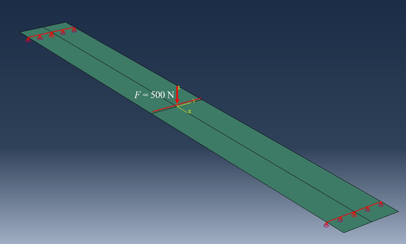
Figure-9: Shell model
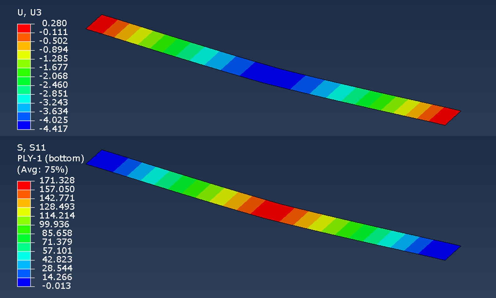
Figure-10: Shell model results
data_shell_t = np.genfromtxt('data/s1-shell-top.txt')
data_shell_b = np.genfromtxt('data/s1-shell-bottom.txt')

fig, (ax1,ax2) = plt.subplots(nrows=1,ncols=2,figsize=(12,4))
ax1.plot(data_shell_t[:,0],data_shell_t[:,1],label='shell')
ax1.plot((-125,0,125),(0,-167,0),label='analytical')
ax1.set_xlabel('x [mm]')
ax1.set_ylabel('Stress [MPa]')
ax1.set_title('Longitudinal stress along top')
ax1.grid(True)
ax1.legend(loc='best')

ax2.plot(data_shell_b[:,0],data_shell_b[:,1],label='shell')
ax2.plot((-125,0,125),(0,167,0),label='analytical')
ax2.set_xlabel('x [mm]')
ax2.set_ylabel('Stress [MPa]')
ax2.set_title('Longitudinal stress along top')
ax2.grid(True)
ax2.legend(loc='best')

plt.tight_layout()
plt.show()

Concluding remarks
- Regarding deflection, the three approaches agrees well.
- The analytical solution and the shell model computes essentially the same values for maximum and minimum longitudinal stress
- Only the solid model is able to capture 3D state of stress at support and load, as expected, and these local effects are obviously important when assessing the strength of the beam.
To be addressed in exercises
- A local compressive strain through the thickness may induce premature failure due to a combination of compressive strength and buckling. Explain the mechanisms.
- This case study demonstrates the importance of compressive strength and stiffness of the core material. Discuss this issue and compare results with properties of similar core material.
- Explain briefly how the shell elements in Abaqus estimate the transverse shear deformation according to the Abaqus Documentation.
- The model for the sandwich beam in this study could obviously be reduced to ¼ by utilizing the perfect symmetry that exists for both geometry, material and layup as well as loading. Investigate how significant a layup [-45/45/core/45/-45] will deviate from symmetry conditions with respect to the mechanical behavior (more details given in the exercise)


