Crossbow
This study focuses on the mechanical performance of the limbs in a traditional crossbow design
The primary function of a crossbow limb is to store elastic strain energy, which is then transferred to the arrow or bolt as kinetic energy upon release.
However, a portion of this strain energy is also converted into kinetic energy within the limb itself, with the magnitude of this transfer dependent on the limb's mass and displacement range. Therefore, to maximize efficiency, the limbs should ideally store as much elastic energy as possible while remaining as lightweight as possible.
A limb is fundamentally a leaf spring. If the objective is to store as much energy as possible per volume material, the material's capacity for elasic strain energy density should be maximized, i.e.
\begin{equation} \max \Big( \frac{\sigma_f^2 }{E}\Big) \tag{1} \end{equation}where $\sigma_f$ is the relevant strength or elastic limit for the material, and $E$ is the Young's modulus in the relevant direction of the material.
Throughout history, crossbow limbs were initially crafted from selected woods. With advancements in metallurgy during the medieval period, high-strength carbon steels began to replace wood, providing greater durability and power.
The development of fiber composites marked a significant leap in efficiency, outperforming traditional materials and now dominating the market for high-performance crossbows, as will be demonstrated numerically:
Let the strength of both the spring steel and an UD-glass fiber composite (GFRP) be 1000 MPa. The respetive material indices and the ratio of GFRP to steel are:
ind_steel = (1000**2)/(200000)
ind_gfrp  = (1000**2)/( 40000)
ratio = ind_gfrp/ind_steel

print('Strain energy capacity per volume, GFRP to Steel ratio: {:.1f}'.format(ratio))
The result shows that GFRP is capable to store 5 times more energy per volume compared to steel.
Even more significant, the ratio is approximatly 20 when comparing energy per mass:
\begin{equation} \max \Big( \frac{\sigma_f^2 }{E \rho}\Big) \tag{2} \end{equation}ind_steel = (1000**2)/(200000*7800)
ind_gfrp = (1000**2)/(40000*2000)
ratio = ind_gfrp/ind_steel
print('Strain energy capacity per mass, GFRP to Steel ratio: {:.1f}'.format(ratio))
Simplified analytical analysis
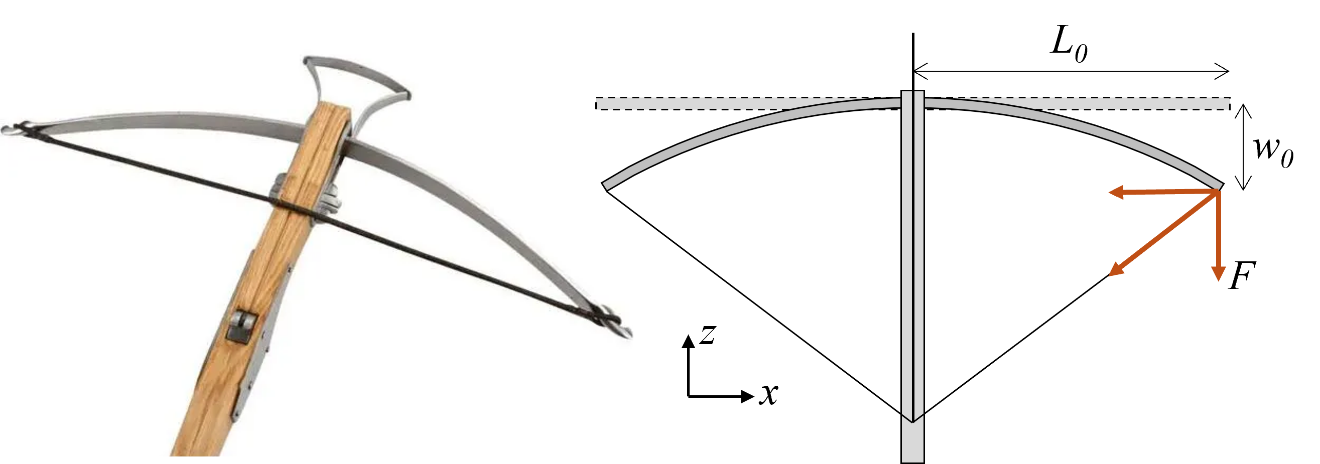
Let one limb be defined by the following constraints illustrated in the figure above:
- The length $L_0$ of the limbs is specified
- The constant width $b_0$ of the limbs is specified
- The draw length is specified, implying that the tip deflection $w_0$ is given
- The stress cannot exceed the failure stress, i.e. $\sigma \le \sigma_f$
- The cross section does not change along $x$
The thickness $h$ is a free variable.
The limb can now be described as a simple cantilever beam with a rectangular cross section where the second moment of area is
\begin{equation} I = \frac{b_0 h^3}{12} \tag{3} \end{equation}The vertical component of force $F$ versus the deflection $w_0$ is:
\begin{equation} F = \frac{3EIw_0}{L_0^3} \tag{4} \end{equation}Moment:
\begin{equation} M = F L_0 \tag{5} \end{equation}Maximum stress:
\begin{equation} \sigma = \frac{h}{2}\frac{M}{I} \tag{6} \end{equation}Requirement:
\begin{equation} \sigma \le \sigma_f \tag{7} \end{equation}The allowable thickness can now be found by solving the relations above. Then, the stored elastic energy is
\begin{equation} U = \frac{1}{2}F w_0 \tag{8} \end{equation}The following code does the job using a simple iterative method (too lazy to manipulate the relations):
def computeCase1(mat, w0, b0, L0, sf, E, rho):
    h_min = 1E-6                    # not less than this...
    h_max = 1E6                     # not greater than this..
    h = 1.0                         # wild guess...
    for i in range(0,1000):         # iterate wildly to find allowable thickness
        I = (b0*h**3)/12            # (3)
        F = (3*E*I*w0)/(L0**3)      # (4)
        M = F*L0                    # (5)
        s = (h/2)*(M/I)             # (6)
        if s>sf:                    # (7)
            h_max = h
        else:
            h_min = h
        h = (h_min+h_max)/2.0
    m = L0*b0*h*rho
    U = 0.5*F*w0                    # (8)
    print('Material: {}: h = {:4.1f} mm,  F = {:6.1f} N, U = {:5.1f} J,  m = {:6.3} kg'.format(mat,h*1000,F,U,m))
    return U, m
Numerical examples:
U1, m1 = computeCase1(mat = 'Steel', w0=200E-3, b0=20E-3, L0=500E-3, sf=1000E6, E=200E9, rho=7800)
U2, m2 = computeCase1(mat = 'GFRP ', w0=200E-3, b0=20E-3, L0=500E-3, sf=1000E6, E= 40E9, rho=2000)
Relative efficiency per mass is in fact identical to the result based on equation (2):
ratio = (U2/m2)/(U1/m1)
print('Strain energy capacity per mass, GFRP to Steel ratio: {:.1f}'.format(ratio))
Alternatively, let the tip deflection be a free variable $w$ while the the thickness $h_0$ is specified. Some minor modifications of the previously developed function:
def computeCase2(mat, b0, L0, sf, E, rho, h0):
    w_min = 1E-6                    # not less than this...
    w_max = 1E6                     # not greater than this..
    w = 1.0                         # wild guess...
    for i in range(0,1000):         # iterate wildly to find allowable deflection
        I = (b0*h0**3)/12           # (3)
        F = (3*E*I*w)/(L0**3)       # (4)
        M = F*L0                    # (5)
        s = (h0/2)*(M/I)            # (6)
        if s>sf:                    # (7)
            w_max = w
        else:
            w_min = w
        w = (w_min+w_max)/2.0
    m = L0*b0*h0*rho
    U = 0.5*F*w                     # (8)
    print('Material: {}: w = {:5.1f} mm,  F = {:6.1f} N, U = {:5.1f} J,  m = {:6.3} kg'.format(mat,w*1000,F,U,m))
    return U, m
U1, m1 = computeCase2(mat = 'Steel', h0=10E-3, b0=20E-3, L0=500E-3, sf=1000E6, E=200E9, rho=7800)
U2, m2 = computeCase2(mat = 'GFRP ', h0=10E-3, b0=20E-3, L0=500E-3, sf=1000E6, E= 40E9, rho=2000)
ratio = (U2/m2)/(U1/m1)
print('Strain energy capacity per mass, GFRP to Steel ratio: {:.1f}'.format(ratio))
Concluding remarks so far
- The material properties are somewhat questionable: There are steels with greater strength to be found, and the applied strength for the GFRP is perhaps somewhat optimistic for a working solution, knowing that the composite is likely to fail by compressive fiber failure where 1000 MPa would require extreemly high quality. The examples shows however the enormous potential of using a material with high strength and low stiffness.
- The material indices in (1) and (2) can be considered generically independent of the geometrical configuration of a leaf spring as illustrated by two different set of constraints.
FEA model